0179
Experimental Realization of Single Current Diffusion Tensor Magnetic Resonance Electrical Impedance Tomography1Electrical and Electronics Engineering Dept., Middle East Technical University (METU), Ankara, Turkey
Synopsis
To obtain low-frequency anisotropic conductivity distribution of biological tissues recently Diffusion Tensor Magnetic Resonance Electrical Impedance Tomography (DT-MREIT), which is combination of the DTI and MREIT techniques, is proposed. There are two in vivo applications of DT-MREIT in the literature where two linearly independent current injection patterns are used. Decreasing the number of current injection patterns to one improves the feasibility of DT-MREIT in clinical applications. In this study, DT-MREIT using a single current injection pattern is experimentally realized. The obtained results approve the validity of the proposed single current DT-MREIT method.
INTRODUCTION
Conductivity tensor images provide a unique contrast for diagnostic purposes. Recently, Diffusion Tensor Magnetic Resonance Electrical Impedance Tomography (DT-MREIT) is proposed in, 1,2 to reconstruct conductivity tensor images of anisotropic biological tissues exploiting the linear relationship between the diffusion ($$$\overline{\overline{D}}$$$) and conductivity ($$$\overline{\overline{C}}$$$) tensors in a porous medium3:$$\overline{\overline{C}}=\eta\overline{\overline{D}}\space\space\space\space\space\space\space\space\space\space(1)$$
where $$$\eta$$$ is the extra-cellular conductivity and diffusivity ratio (ECDR). There are two in vivo applications of DT-MREIT in the literature4,5 where two linearly independent current injection patterns are used to reconstruct $$$\eta$$$. The reported results present high resolution cross-sectional conductivity tensor images of canine and human brains. To improve clinical practicality of DT-MREIT reducing the total scan time is desired. By using only a single current injection pattern not only the scan time is improved but also by reducing the number of current injection cables and contact electrodes to half, the patient comfort increases during data acquisition. In this study, single current DT-MREIT is realized using an experimental phantom with anisotropic inhomogeneities and the obtained results are presented.
METHODS
The mathematical background of the conventional two current DT-MREIT is given in, 2. To reconstruct $$$\eta$$$ using a single current injection first-order discrete approximations of $$$x$$$ and $$$y$$$ gradient operators i.e. $$$\overline{\overline{\delta}}_x$$$ and $$$\overline{\overline{\delta}}_y$$$6,7 are utilized. By considering the generalized form of the Ohm’s law:$${\overline{J_{p}}}=-\overline{\overline{C}}{\nabla\phi}=-\eta\overline{\overline{D}}{\nabla\phi}\space\space\space\space\space\space\space\space\space\space(2)$$
and using the curl-free condition of the electric filed at low frequencies, the forward problem of DT-MREIT for a single current injection can be expressed as:
$$\tilde{\nabla}\times(\overline{\overline{D}}\space^{-1}{\overline{J}_{p}})=\tilde{\nabla}ln(\eta)\times(\overline{\overline{D}}\space^{-1}\overline{J}_p)\space\space\space\space\space\space\space\space\space\space(3)$$
In Eq.2-3, $$$\overline{J}_{p}$$$ is the projected current density8, $$$\phi$$$ is the scalar electrical potential corresponding to $$$\overline{J}_{p}$$$ and $$$\tilde{\nabla}=(\frac{\partial}{\partial{x}},\frac{\partial}{\partial{y}})$$$. Eq.3 can be expressed in matrix form for each pixel as:
$$\begin{bmatrix}(\overline{\overline{D}}\space^{-1}{\overline{J}_{p}})_y&-(\overline{\overline{D}}\space^{-1}{\overline{J}_{p}})_x\end{bmatrix}_{1\times2}\begin{bmatrix}\frac{\partial{ln(\eta)}}{\partial{x}}\\\frac{\partial{ln(\eta)}}{\partial{y}}\end{bmatrix}_{2\times1}=\begin{bmatrix}\frac{\partial(\overline{\overline{D}}\space^{-1}{\overline{J}_{p}})_x}{\partial{y}}&-\frac{\partial(\overline{\overline{D}}\space^{-1}{\overline{J}_{p}})_y}{\partial{x}}\end{bmatrix}_{1\times1}\space\space\space\space\space\space\space\space\space\space(4)$$
Eq.4 can be expanded for the imaged slice which composed of $$$N$$$ pixels as:
$$\overline{\overline{A}}_{N\times{N}}ln(\overline{\eta})_{N\times1}=\overline{c}_{N\times1}\space\space\space\space\space\space\space\space\space\space(5)$$
where
$$\overline{\overline{A}}=diag(\overline{a}_1)\overline{\overline{\delta}}_x+diag(\overline{a}_2)\overline{\overline{\delta}}_y,\\\overline{a}_1=\begin{bmatrix}(\overline{\overline{D}}\space^{-1}{\overline{J}_{p}})_{y,1}\\\vdots\\(\overline{\overline{D}}\space^{-1}{\overline{J}_{p}})_{y,N}{}\end{bmatrix}_{N\times1},\space\space\space\space\space\overline{a}_2=\begin{bmatrix}(\overline{\overline{D}}\space^{-1}{\overline{J}_{p}})_{x,1}\\\vdots\\(\overline{\overline{D}}\space^{-1}{\overline{J}_{p}})_{x,N}{}\end{bmatrix}_{N\times1},\\\overline{c}=\begin{bmatrix}{(\frac{\partial(\overline{\overline{D}}\space^{-1}{\overline{J}_{p}})_x}{\partial{y}}-\frac{\partial(\overline{\overline{D}}\space^{-1}{\overline{J}_{p}})_y}{\partial{x}})_1}\\\vdots\\{(\frac{\partial(\overline{\overline{D}}\space^{-1}{\overline{J}_{p}})_x}{\partial{y}}-\frac{\partial(\overline{\overline{D}}\space^{-1}{\overline{J}_{p}})_y}{\partial{x}})_N}{}\end{bmatrix}_{N\times1}\space\space\space\space\space\space\space\space\space\space(6)$$
and $$$diag(\overline{v})$$$ returns a square diagonal matrix with $$$\overline{v}$$$ as the main diagonal. In Eq.5, $$$\overline{\eta}$$$ is the vector composed of scalar $$$\eta$$$ values of all pixels in the imaged slice. Each entry of $$$\overline{a}_1$$$, $$$\overline{a}_2$$$ and $$$\overline{c}$$$ are obtained from a single pixel in the imaged slice. To solve Eq.5, Transpose Free Quasi-Minimal Residual method (TFQMR)9 is utilized due to sparsity of $$$\overline{\overline{A}}$$$.
EXPERIMENTAL SETUP
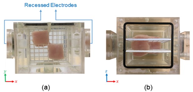
The data acquisition is performed using a 3T MRI scanner (MAGNETOM Trio, Siemens AG, Erlangen, Germany) equipped with a 32 channel head coil.The experimental phantom is a 3D Plexiglas container with the dimensions of $$$80\times80\times80\space{}mm^3$$$ filled with a saline solution with the conductivity and $$$T_2^*$$$ values of $$$0.5\space{}S/m$$$ and $$$180\space{}ms$$$ which approximately mimic the human blood10,11. Two pieces of chicken muscle are used as anisotropic inhomogeneities and placed at the middle slice of the phantom as shown in Fig.1. A custom-designed current source12 is used to produce current pulses in synchrony with the MR pulse sequence.
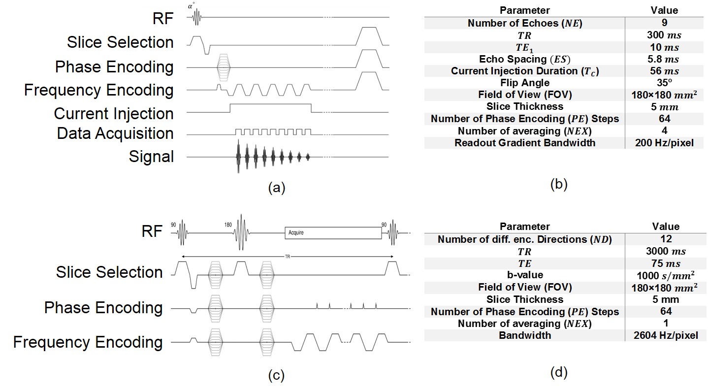
For MREIT data acquisition Induced Current Nonlinear Encoding Spoiled Multi Gradient Echo (ICNE-SPMGE) pulse sequence in Fig.2(a) is utilized. On the other hand, Single Shot Spin-Echo EPI (SS-SE-EPI) pulse sequence in Fig.2(b) is used for the DTI data acquisition procedure.
RESULTS
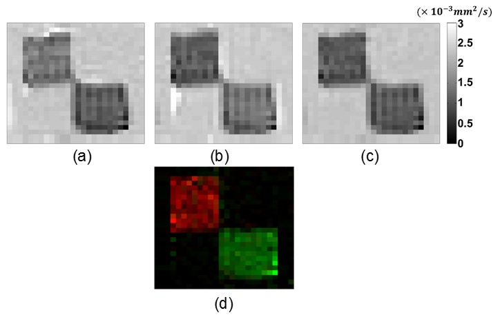
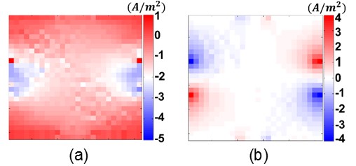
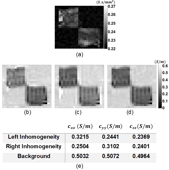
The main diagonal elements of DT with Fractional Anisotropy (FA) map and the projected current density distributions of the experimental phantom are shown in Fig.3-4, respectively.Using the DT and the projected current density data in Fig.3-4 the ECDR ($$$\eta$$$) distribution of the experimental phantom is obtained by means of the proposed method in Eq.5 and shown in Fig.5(a). The reconstructed main diagonal elements of the conductivity tensor for the experimental phantom using the relation in Eq.1 are shown in Fig.5(b-d).
DISCUSSION
Considering $$$c_{xx}^{left}\approx{}c_{yy}^{right},\space{}c_{yy}^{left}\approx{}c_{xx}^{right},\space{}c_{zz}^{left}\approx{}c_{zz}^{right}$$$ and bearing in mind the orientations of muscle fibers (the fibers of the left and right chicken muscles are aligned with $$$x$$$ and $$$y$$$ directions, respectively), it can be seen that the proposed method reconstructs realistic ratios of anisotropic conductivity values. Moreover, the reconstructed mean value of the background material with isotropic distribution is consistent with the assigned conductivity value of the saline solution ($$$0.5\space{}S/m$$$). Hence, it can be inferred that the proposed method successfully reconstructs the conductivity distributions of the experimental phantom using only a single current injection pattern. Decreasing the number of linearly independent patterns to one reduces both the data acquisition duration and number of current injection cables and contact electrodes to half. The reduction of data acquisition duration reduces image artifacts related to patient motion and respiration. On the other hand, the less number of current injection cables and contact electrodes enhances the clinical practicality of DT-MREIT. Furthermore, both reductions improve patient comfort. These implications become even more significant when a high number of averaging is utilized in order to obtain higher SNR levels which require longer imaging time.CONCLUSION
In this study, practical implementation of a single current DT-MREIT method which is proposed to increase the clinical practicality of DT-MREIT is conducted. The results show that good contrast and realistic conductivity values can be reconstructed by one current administration. This is the first study that the anisotropic conductivity distribution is obtained experimentally with only one current injection. This improvement carries the importance of making the DT-MREIT method more feasible in clinical applications. Future studies may include in vivo experiments to justify these aspects further.Acknowledgements
This work is a part of the Ph.D. thesis study of Mehdi Sadighi. B. Murat Eyüboğlu is the thesis supervisor. Mert Şişman and Berk Can Açıkgöz are graduate students under the supervision of B. Murat Eyüboğlu.
This study is funded by The Scientific and Technological Research Council of Turkey (TÜBİTAK) under Research Grant 116E157.
Experimental data were acquired using the facilities of UMRAM (National Magnetic Resonance Research Center), Bilkent University, Ankara, Turkey.
References
1. Ma W, DeMonte TP, Nachman AI, Elsaid NM, Joy ML. Experimental implementation of a new method of imaging anisotropic electric conductivities. In2013 35th Annual International Conference of the IEEE Engineering in Medicine and Biology Society (EMBC) 2013 Jul 3 (pp. 6437-6440).
2. Kwon OI, Jeong WC, Sajib SZ, Kim HJ, Woo EJ. Anisotropic conductivity tensor imaging in MREIT using directional diffusion rate of water molecules. Physics in Medicine & Biology. 2014 May 19;59(12):2955-2974.
3. Tuch DS, Wedeen VJ, Dale AM, George JS, Belliveau JW. Conductivity tensor mapping of the human brain using diffusion tensor MRI. Proceedings of the National Academy of Sciences. 2001 Sep 25;98(20):11697-11701.
4. Jeong WC, Sajib SZ, Katoch N, Kim HJ, Kwon OI, Woo EJ. Anisotropic conductivity tensor imaging of in vivo canine brain using DT-MREIT. IEEE transactions on medical imaging. 2016 Aug 8;36(1):124-131.
5. Chauhan M, Indahlastari A, Kasinadhuni AK, Schär M, Mareci TH, Sadleir RJ. Low-Frequency Conductivity Tensor Imaging of the Human HeadIn VivoUsing DT-MREIT: First Study. IEEE transactions on medical imaging. 2017 Dec 14;37(4):966-976.
6. Sharif B, Kamalabadi F. Optimal sensor array configuration in remote image formation. IEEE Transactions on Image Processing. 2008 Jan 14;17(2):155-166.
7. Hansen PC. Discrete inverse problems: insight and algorithms. Siam; 2010 Mar 18.
8. Park C, Lee BI, Kwon OI. Analysis of recoverable current from one component of magnetic flux density in MREIT and MRCDI. Physics in Medicine & Biology. 2007 May 4;52(11):3001-3013.
9. Freund RW. Transpose-free quasi-minimal residual methods for non-Hermitian linear systems. In Recent advances in iterative methods 1994 (pp. 69-94). Springer, New York, NY.
10. Gabriel C, Peyman A, Grant EH. Electrical conductivity of tissue at frequencies below 1 MHz. Physics in medicine & biology. 2009 Jul 27;54(16):4863-4878.
11. Cistola DP, Robinson MD. Compact NMR relaxometry of human blood and blood components. TrAC Trends in Analytical Chemistry. 2016 Oct 1;83:53-64.
12. Eroglu HH, Eyüboglu BM, Göksu C. Design and implementation of a bipolar current source for MREIT applications. InXIII Mediterranean Conference on Medical and Biological Engineering and Computing 2013 2014 (pp. 161-164). Springer, Cham.
Figures