INTRODUCTION:

Transcranial electrical stimulation (tES) is a non-invasive neuromodulation technique indicated to treat depression and chronic pain¹. In tES, low amplitude current is delivered to the brain through surface electrodes². The best contemporary estimates of electric fields delivered by tES are estimated from computational models of the head³. However, these models rely on literature values for tissue conductivities and do not include electrode contact impedances. Therefore, this approach cannot correctly predict subject-specific fields. DT-MREIT⁴ has recently been introduced to produce electrical conductivity tensor images by imaging of a scale factor ($$$\eta$$$) relating MRI diffusion and conductivity tensors. Stable reconstruction of $$$\mathbf{C}$$$ via DT-MREIT requires two independent current administrations. Here, we use data from an in-vivo human experiment to demonstrate that it is possible to reconstruct $$$\mathbf{C}$$$ using a single experimental current administration.

METHODS:

Experiment: Experimental protocols were approved by the Arizona State University Institutional Review Board. Data obtained from a 58-year old volunteer male human subject was used to demonstrate method performance. Data were measured using a 32-channel RF head coil in a 3.0T Phillips scanner (Phillips, Ingenia, Netherlands) located at the Barrow Neurological Institute (Phoenix, Arizona, USA). A transcranial electrical stimulator (DC-STIMULATOR MR, neuroConn, Ilmenau, Germany) was used to deliver 1.5 mA currents using an Fpz-Oz electrode montage. Sets of $$$B_z^m$$$ data were measured on three axial slices using a multi-echo gradient-echo pulse sequence and an image matrix size of 128$$$\times$$$128. Other imaging parameters were, TR/TE/ES=50/7/3 ms, FOV= 224$$$\times$$$ mm², slice thickness, 5 mm, and number of echoes, NE = 10. Individual echo images were then combined to improve the SNR of the acquired $$$B_z^m$$$ signal⁵. Prior to echo combination, stray magnetic field corrections were applied to each echo image⁶. Figure 1 (b) and (d) show acquired MR magnitude and echo-combined $$$B_z^{opt}$$$ images respectively for the center slice. Diffusion-weighted images of the three MREIT slices were also obtained, using an SS-SE-EPI imaging sequence, with $$$b$$$ of 1000 sec/mm² and fifteen diffusion directions. The FA map is shown in Fig. 1(e). High-resolution T1-weighted images were also collected to construct computational models of the head and lead wires (Fig 1a).

Scale-factor reconstruction: We applied the KVL in a rectangular region $$$\Omega_{ij}$$$, $$$\Omega_{ij}^{'} \in \Omega_t$$$ where, $$$\Omega_t$$$ is the DT-MREIT slice at $$$z=t$$$ (Fig. 2b). A dual-loop relationship relating the water diffusion tensor $$$\mathbf{D}$$$, estimated regional current density⁷ $$$\mathbf{J}^{P}$$$ from experimentally obtained $$$B_z^{opt}$$$ data and the target $$$\hat{\eta}$$$ was formulated as

$$\begin{cases}\frac{\left(\mathbf{D}^{-1}\mathbf{J}^P\right)_x\left(p_{ij,1}\right)}{\hat{\eta}(x_i,y_{j-1})}+\frac{\left(\mathbf{D}^{-1}\mathbf{J}^P\right)_y\left(p_{ij,2}\right)}{\hat{\eta}(x_i,y_j)}-\frac{\left(\mathbf{D}^{-1}\mathbf{J}^P\right)_x\left(p_{ij,3}\right)}{\hat{\eta}(x_i,y_j)}-\frac{\left(\mathbf{D}^{-1}\mathbf{J}^P\right)_y\left(p_{ij,4}\right)}{\hat{\eta}(x_{i-1},y_j)}=0&\mbox{in}~\Omega_{ij}\\\frac{\left(\mathbf{D}^{-1}\mathbf{J}^P\right)_x\left(p^{'}_{ij,1}\right)}{\hat{\eta}(x_i,y_j)}+\frac{\left(\mathbf{D}^{-1}\mathbf{J}^P\right)_y\left(p^{'}_{ij,2}\right)}{\hat{\eta}(x_{i+1},y_j)}-\frac{\left(\mathbf{D}^{-1}\mathbf{J}^P\right)_x\left(p^{'}_{ij,3}\right)}{\hat{\eta}(x_i,y_{j+1})}-\frac{\left(\mathbf{D}^{-1}\mathbf{J}^P\right)_y\left(p^{'}_{ij,4}\right)}{\hat{\eta}(x_i,y_j)}=0&\mbox{in}~\Omega^{'}_{ij}\end{cases} (1) $$

Scale factor values at the boundary were assumed, and an overdetermined system was built comprising $$$2\left(N-2\right)^2$$$ equations, which was then solved for $$$\left(N-2\right)^2$$$ internal nodes.

Dual-loop $$$\hat{\eta}$$$ reconstructions were affected by streaking artefacts due to noise propagation along equipotential lines (Fig. 3b left). To overcome this, a regressor model of non-linear artefact functions was built using a deep neural network^8,9 (Fig. 2a). Training datasets were obtained from numerical simulations only. Scale factor values were assumed piecewise constant in each tissue (GM, WM, CSF), and the DT-MREIT forward problem⁴ was been solved for 1000 numerical models (WM: 0.2-0.775, GM: 0.2-0.775, CSF: 0.4-0.8 S•sec/mm³ with 0.1 S•sec/mm³ linear step) using an FPz-Oz electrode montage. Noise of 0.21 nT was added to each simulated $$$B_z^{*}$$$ image¹⁰. Artefact-affected $$$\eta^{*}$$$ images were then reconstructed using (1). Data from a complementary electrode montage (T7-T8) was simulated and used to reconstruct artifact-free images of $$$\tilde{\eta}^{*}$$$ using the two-current injection DT-MREIT method⁴ (Fig. 2c). These two training datasets were used to train a U-net architecture (Fig. 2a) implemented in Keras library in Python. By minimizing $$$l^2$$$ loss function, 1,327,744 parameters were trained using the RMSProp optimizer with 32-mini-batch size and 1000 epochs.

Electric field reconstruction: The conductivity tensor $$$\mathbf{C} = \eta \mathbf{D}$$$ was calculated using scale-factors from the trained network (Fig. 2a). Electric field distributions were then estimated using $$$\mathbf{E} = \mathbf{C}^{-1} \mathbf{J}^P$$$.

Verification: Reconstruction performance was verified using relative $$$L^2$$$-differences from standard scale-factor images obtained using the DT-MREIT algorithm³ and another set of $$$B_z^m$$$ data measured using a T7-T8 electrode pair.

RESULTS:

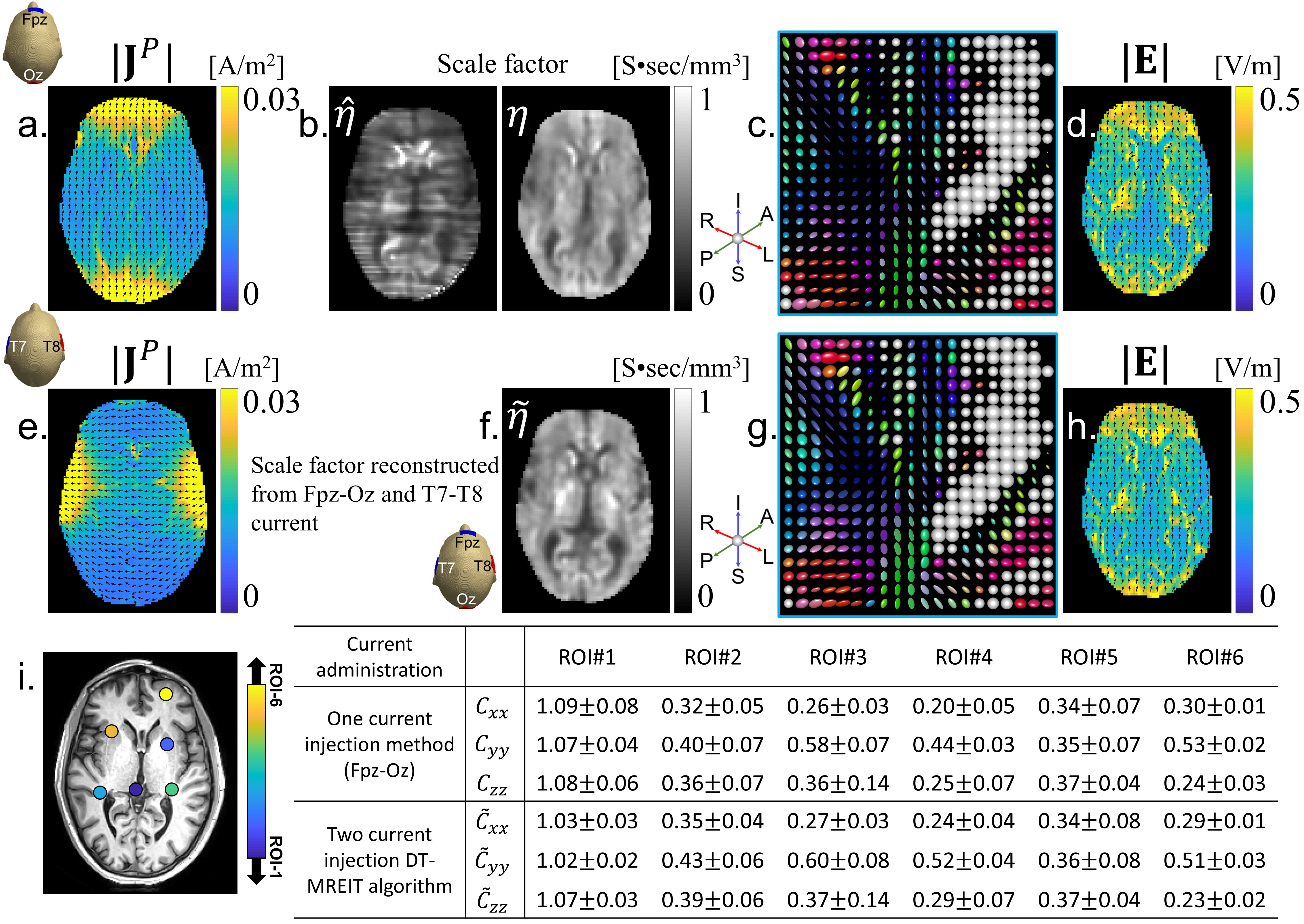
Figure 3(a) shows estimated projected current density caused by current flow through the Fpz-Oz electrode montage. Reconstructed scale factor images from (1) are in Fig. 3(b-left). As expected, the reconstructed scale factor image from one current injection was corrupted by streaking artefacts. Results obtained after correction using the deep neural network (Fig. 2a) are in Fig. 3(b-right). The neural-network corrected scale factor image was multiplied with measured diffusion tensor data to form conductivity tensors⁴ (Fig. 3(c)) shows the reconstructed tensor within the ROI (Fig. 1b). Reconstructed electric fields are shown in Fig. 3d and compared with those from the two-current administration method4 (Fig. 3e-i). Relative $$$L^2$$$-differences between single-current injection and standard-reconstructed $$$\eta$$$ and derived electric fields were found to be 0.15 and 0.20 respectively.

DISCUSSION:

We have demonstrated that it is possible to reconstruct the conductivity tensor with reasonable accuracy using single current data. One of the drawbacks of this implementation is the limited number of training datasets. We plan to use this method to reconstruct the electromagnetic field for F3-F4 electrode montages using larger numbers of training datasets.

CONCLUSIONS:

Results of in-vivo human experiments demonstrate that stable conductivity tensors can be reconstructed using only one current injection.

Acknowledgements

This work was supported by award RF1MH114290 to RJS.