Introduction

For studying electromagnetic tissue properties [1], EPT [2] reconstructs conductivity from transceive B1 phase data without B1 magnitude mapping, and QSM [3] retrieves tissue’s magnetic susceptibility from B0 field data typically estimated from multi-echo GRE (mGRE) signal. In a traditional phase based EPT, the transceive B1 phase is obtained from spin echo (SE) acquisition, which is free from B0 inhomogeneity effect and reflects only B1-related phase. Several studies show that transceiver B1 phase can also be estimated from mGRE signal by extrapolating phase evolution along echo time [4]. In this paper, we estimate B1 phase and B0 field distributions simultaneously from mGRE signal by applying nonlinear least squares on the complex signal equation [5], which can achieve the maximum likelihood estimation.

Method

Since EPT assumes that both transmit and receive B1 magnitude fields are sufficiently homogeneous to retrieve conductivity from B1 phase information, individual coil’s data were properly combined to minimize receive B1 magnitude variation [6,7] as follows. Receiver coil sensitivities $$$B_{1,j}^{-}$$$ were first estimated using ESPIRiT method [8], and then combination coefficients $$$c_{j}(\boldsymbol{r})$$$ were determined by minimizing combined receive B1 field variation:
$$c_{j}(\boldsymbol{r})=\mathrm{argmin}_{c_{j}(\boldsymbol{r})}\|\sum_{j = 1}^{N}B_{1,j}^{-}c_{j}(\boldsymbol{r})-1\|_{2}^{2}+\lambda\sum_{j = 1}^{N}|c_{j}(\boldsymbol{r})|^{2},$$
where norm was taken inside the neighboring region of each point . Next, B1 phase as well as B0 field were estimated according to Gaussian noise model in complex mGRE data:
$$\phi,\Delta B_{0}=\mathrm{argmin}_{\phi,\Delta B_{0}}\|S(T_{E})-\rho\exp(-R_{2}^{\ast}T_{E})\exp(\mathrm{i}(\phi-\gamma\Delta B_{0}T_{E}))\|_{2}^{2},$$
where $$$\rho$$$ is proton density, $$$R_{2}^{\ast}$$$ is relaxation rate, $$$\gamma$$$ is gyromagnetic ratio, and $$$T_{E}$$$ is echo time. The summation is over the all echoes. Minimization was conducted by the Levenberg–Marquardt method. To compare B1 phase estimated from mGRE with SE phase, two FSE images with opposite readout gradients were also acquired and averaged to yield the gold standard phase image.
Once coil-combined B1 phase image was obtained, its Laplacian was calculated using Savitzky-Golay filter, which is based on the second order weighted polynomial fitting in each local region around the voxel of interest. Kernel size was 15x15x5 voxels and the weighting factor was determined from magnitude image as follows: $$$w(\boldsymbol{r}) = G(|I(\boldsymbol{r}) - I(\boldsymbol{r}_{0})|)$$$, where $$$G$$$ represents Gaussian function [7]. Finally, conductivity $$$\sigma$$$ was reconstructed as follows:
$$\sigma=\mathrm{argmin}_{\sigma}\|\sigma-\Delta\phi/(2\omega_{0}\mu_{0})\|_{2}^{2}+\lambda\|M(\nabla I)\nabla\sigma\|_{1},$$
where $$$M(\nabla I)$$$ represents the mask that removes boundaries of different anatomical regions and is used in morphology enabled dipole inversion (MEDI) method [9] in QSM. QSM was also reconstructed using nonlinear MEDI with automatic uniform cerebrospinal fluid zero reference (MEDI+0) [10]. This electromagnetic tissue property estimation from mGRE complex signal is referred to as quantitative conductivity and susceptibility mapping (QCSM).
MRI acquisitions were performed on 5 healthy human subjects and brain data were obtained using 2D FSE and 3D mGRE in a 3T clinical scanner (MR750, GE Healthcare, Waukesha, WI). A 32-channel head coil was used as the receiver coil. The imaging parameters for mGRE were as follows: TR: 53.2 ms, first TE: 4.4 ms, echo spacing: 4.9 ms, flip angle: 15 deg; and for FSE : TR: 5350 ms, eff. TE: 87.9 ms, echo train length: 24, flip angle: 111 deg, NEX: 2. FOV was 240x240x144 mm³ and voxel size was 0.4688x0.4688x3 mm³ for both sequences. QCSM was generated from mGRE data. We also tested the proposed QCSM method with 5 tumor patients’ mGRE data.

Results and Discussion

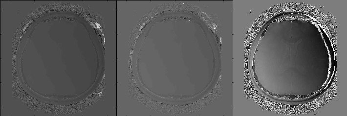
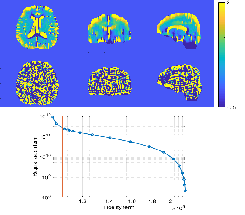
Figure 1 shows the estimated transceiver B1 phase of one representative subject. The estimated B1 phase maps were similar in both linear extrapolation method (left) and in the proposed nonlinear least square method (center). Although B1 phase is less smooth compared with SE phase (right) in both linear and nonlinear methods, the proposed method yielded relatively stable results compared with the linear extrapolation method. This is because the proposed method correctly accounted for the noise distribution and achieves maximum likelihood estimation.
Figure 2 shows the conductivity maps reconstructed from B1 phase estimated by the nonlinear least square method. We varied the regularization parameter and chose the one that maximizes the curvature of L-curve plot shown in Fig.2 (bottom). When no regularization is adopted (middle), the conductivity map is suffered from severe noise. When the anatomical image is utilized as a regularizer (top), the conductivity results are less noisy and anatomical structures are discernible.
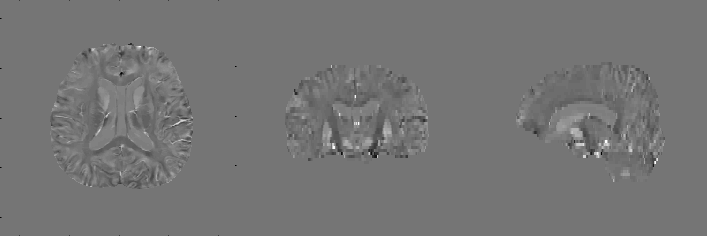
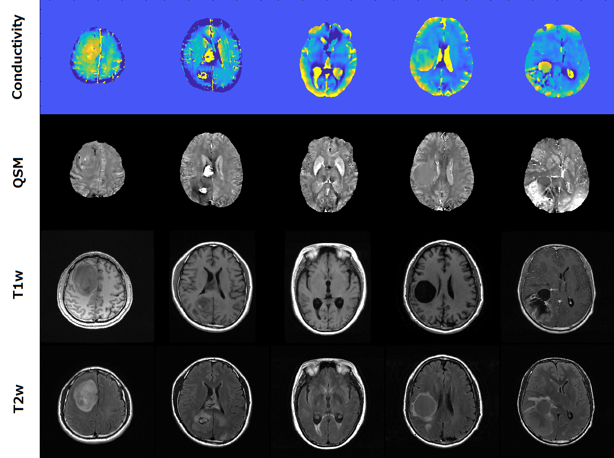
Simultaneously, we obtained B0 field map by solving Eq.2 and reconstructed QSM (Fig.3). This means that electromagnetic tissue properties can be successfully obtained from a single mGRE acquisition. Figure 4 shows the reconstructed conductivity and susceptibility maps along with T1w (3^rd row) and T2w (bottom row) images for 5 tumor patients’ data. The structures of lesions are consistent between conductivity and susceptibility maps, but the conductivity maps have higher values in all cases. Therefore, conductivity maps can give additional pathological information.

Conclusion

We describe a simultaneous quantitative conductivity and susceptibility mapping (QCSM) method by estimating B1 phase and B0 field distributions from multi-echo gradient echo (mGRE) signal. B1 phase and B0 filed maps are simultaneously estimated by applying nonlinear least square method on the complex signal equation of the multi-echo GRE signal. Then, conductivity and susceptibility are reconstructed by incorporating anatomical information as a regularizer. QCSM is feasible and promising for studying electromagnetic tissue properties in healthy brains and in brains with tumors using a single mGRE acquisition.

Acknowledgements

No acknowledgement found.