Introduction

Multi-echo GRE myelin water imaging (MWI) infers white matter (WM) myelination by fitting the multi-echo signal to a 3-pool model¹. This fitting is ill-conditioned because of the similar relaxation times and frequency shifts between the various compartments. Recent DWI development on WM microstructure modelling allows the estimation of not only fibre orientation but also the volume of intra-/extra-cellular water^2,3. Integrating DWI with physics informed signal models has the potential to improve myelin water fraction (MWF) measurements.

Theory

Standard GRE-MWF model considers 3 water pools in WM¹, including myelin water (MW), intra-axonal water (IW) and extracellular water (EW):
$$S\left(t\right)=\left[A_{MW}e^{\left(-R_{2,MW}^{*}+i\omega_{MW}\right)t}+A_{IW}e^{\left(-R_{2,IW}^{*}+i\omega_{IW}\right)t}+A_{EW}e^{\left(-R_{2,EW}^{*}+i\omega_{EW}\right)t}\right]e^{i\left(\omega_{b}t+\phi\right)}[Eq.1]$$
Each pool has distinct signal intensity $$$A$$$, transverse relaxation rate $$$R_{2}^{*}$$$ and frequency shift $$$\omega$$$, while $$$\omega_{b}$$$ and $$$\phi$$$ represent the background field and phase offset.

Hollow cylinder model (HCM) has been used to describe the frequency shifts of MW and IW introduced by the isotropic and anisotropic magnetic susceptibility of the myelin sheath ($$$\chi_{I}$$$ and $$$\chi_{A}$$$)⁴. These are given by:
$$\omega_{MW}=\left[\frac{\chi_{I}}{2}\left(\frac{2}{3}-\sin^{2}\theta\right)+\frac{\chi_{A}}{2}\left(c\sin^{2}\theta-\frac{1}{3}\right)+E\right]{\gamma}B_{0}[Eq.2]$$
$$\omega_{IW}=\frac{3\chi_{A}\sin^{2}\theta}{4}\ln\left(\frac{1}{g}\right){\gamma}B_{0}[Eq.3]$$
where $$$c=1/4-\left(3/2\right)\left(g^{2}/(1-g^{2})\right)\ln{(1/g)}$$$; $$$\theta$$$ is the angle between the fibre and the $$$B_{0}$$$ directions (can be derived from DWI); $$$g$$$ is the ratio between inner and outer axonal radii, but can be derived from $$$g=\sqrt{A_{IW}/\left(A_{IW}+A_{MW}/\rho_{MW}\right)}$$$, and $$$\rho_{MW}$$$ is the relative myelin water density⁵. Therefore, the frequency shifts can be computed from the MWI model without fitting extra parameters when we assume the myelin sheath properties are constants throughout the brain ($$$\chi_{I}=\chi_{A}=-0.1ppm, \rho_{MW}=0.43, E=0.02ppm$$$)^4,5. The same formalism predicts the decay of EW as the sum of the IW $$$R_{2}^{*}$$$ and an extra dephasing effect, $$$D_{E}$$$, due to the inhomogeneous field⁴.

Multi-compartment diffusion models such as NODDI² and spherical mean technique (SMT)³ can estimate the volume fraction of intra-axonal water ($$$v_{ic}$$$). This information can be added to the MWI model as:
$$S\left(t\right)=\left[A_{MW}e^{\left(-R_{2,MW}^{*}+i\omega_{MW}\right)t}+A_{IEW}\left(v_{ic}e^{\left(-R_{2,IW}^{*}+i\omega_{IW}\right)t}+\left(1-v_{ic}\right)e^{\left(-R_{2,IW}^{*}+i\omega_{EW}\right)t}e^{-D_{E}}\right)\right]e^{i\left(\omega_{b}t+\phi\right)}[Eq.4]$$
where $$$A_{IEW}=A_{IW}+A_{EW}$$$.

Methods

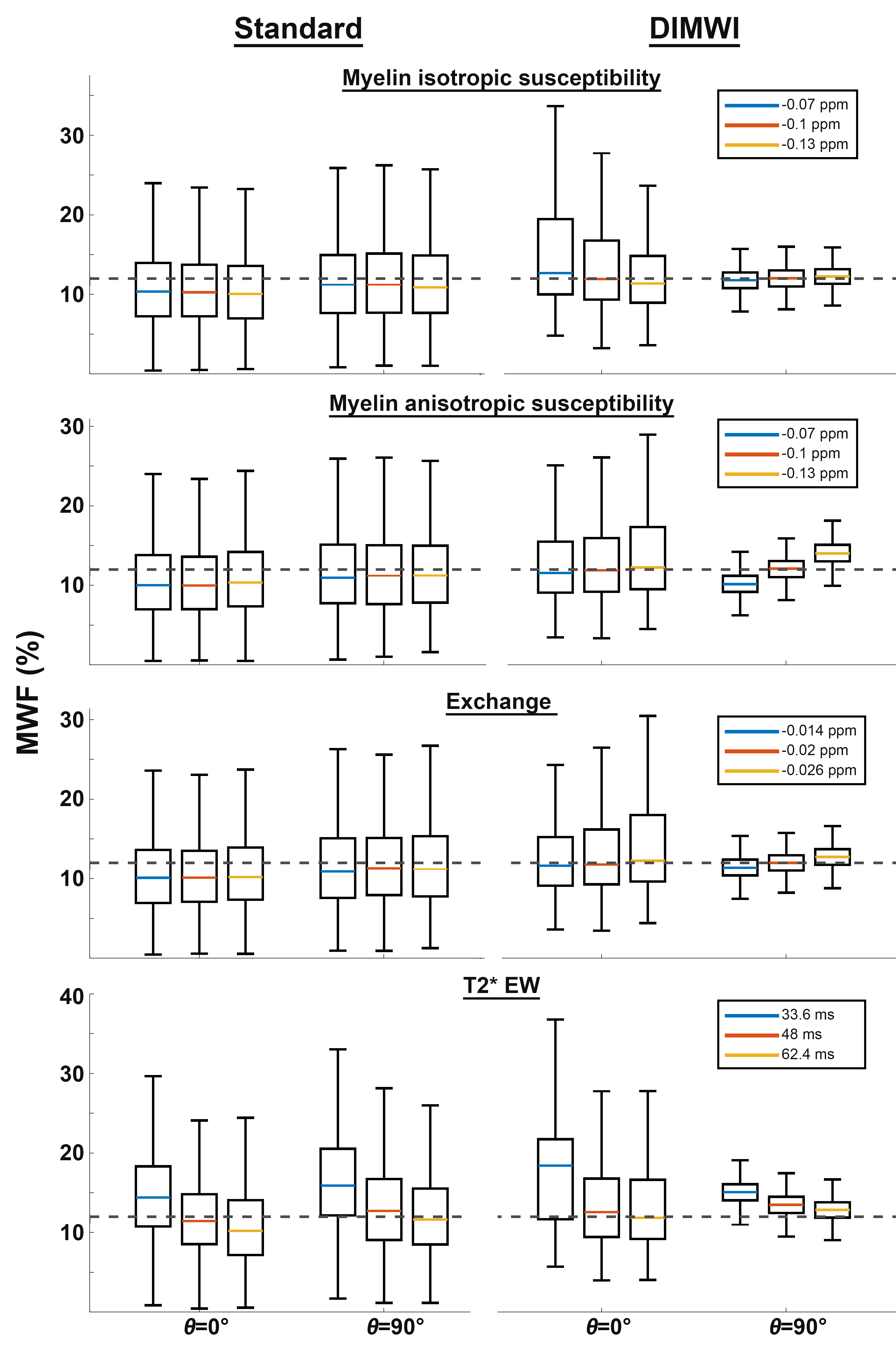
Simulation
Monte Carlo simulations were conducted to study the bias and precision of MWF estimation. 2000 simulations of a 3-pool WM signal⁴ (with the parameters described above) with added Gaussian noise were fitted with the standard and diffusion informed (DIMWI) models. The process was repeated while varying the fixed parameters ($$$\chi_{I}$$$, $$$\chi_{A}$$$, $$$\rho_{MW}$$$ and $$$R_{2}^{*}$$$) in the HCM, assuming under (-30%) or over-estimation (+30%) of those quantities.

In vivo Imaging
All scans were conducted at 3T (Siemens, Erlangen, Germany). Six healthy subjects were scanned with the following protocol:
1) 3D mGRE, TR/TE1/ΔTE/TE12=46/2.15/3.05/35.7ms, res=1.8mm isotropic, α=20° and TA=3.5mins. Repeated 7 times;
2) 2D-MB EPI-DWI, MB=3, res=1.6mm isotropic, TR/TE=3350/71.20ms, 2-shell (b=0/1250/2500 s/mm2, 17/120/120 measurements), TA=15mins.
Two subjects were scanned with the above protocol and a higher resolution GRE sequence:
3) 3D mGRE, TR/TE1/ΔTE/TE12=46/2.15/3.03/35.48ms, res=1.4mm isotropic, α=20° and TA=4.5mins.

DWI was processed with SMT⁴ and a ball-and-stick model⁶ (3 sticks per pixel were allowed) to compute the axonal volume fraction and fibre orientations. MWF maps were computed by fitting the standard (10 parameters) and DIMWI (6 parameters) models on either 1 or averaging of 7 measurements.

Data Analysis
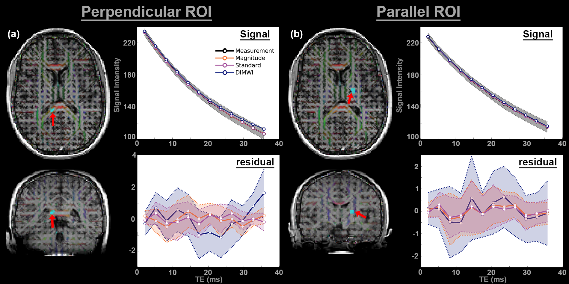
Regions of interest (ROI) were drawn on the splenium of the corpus callosum (26 voxels) and corticospinal tract (30 voxels) of 1 subject. Voxel-wise fitting was performed with a magnitude model (standard model with only signal amplitudes and $$$R_{2}^{*}$$$s, 6 parameters), the standard and the DIMWI models. The mean and standard deviation of the fitting residual was subsequently derived.

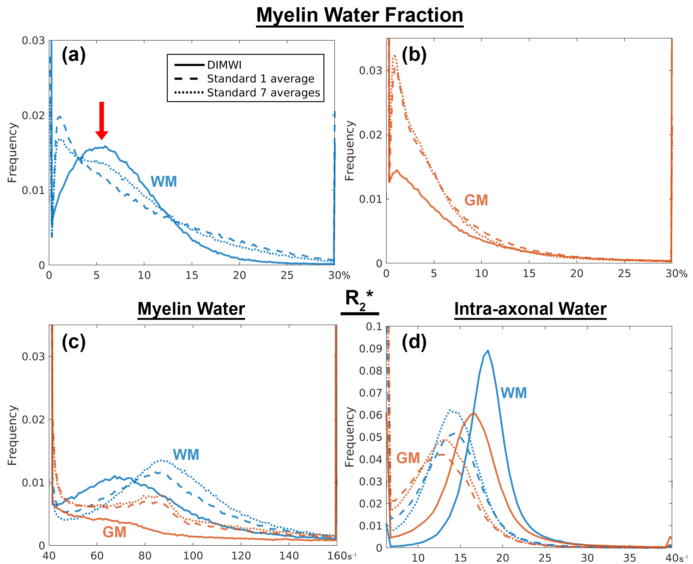
The robustness of the most relevant parameters (MWF and $$$R_{2}^{*}$$$s) of each model was evaluated on their group-averaged histograms within WM and grey matter (GM) masks.

Results and Discussion

The Monte Carlo simulations showed when fibres are not parallel to $$$B_{0}$$$, DIMWI reduced bias and improved precision despite the assumptions of the fixed parameters were invalid (Fig.1).

The ROI analysis demonstrated that the fitting residual of all models is smaller than the standard deviation of the signal (Fig.2). This was the case even the compartmental frequencies were ignored, which is deviated from the HCM prediction, suggesting that MWI is susceptible to over-fitting.

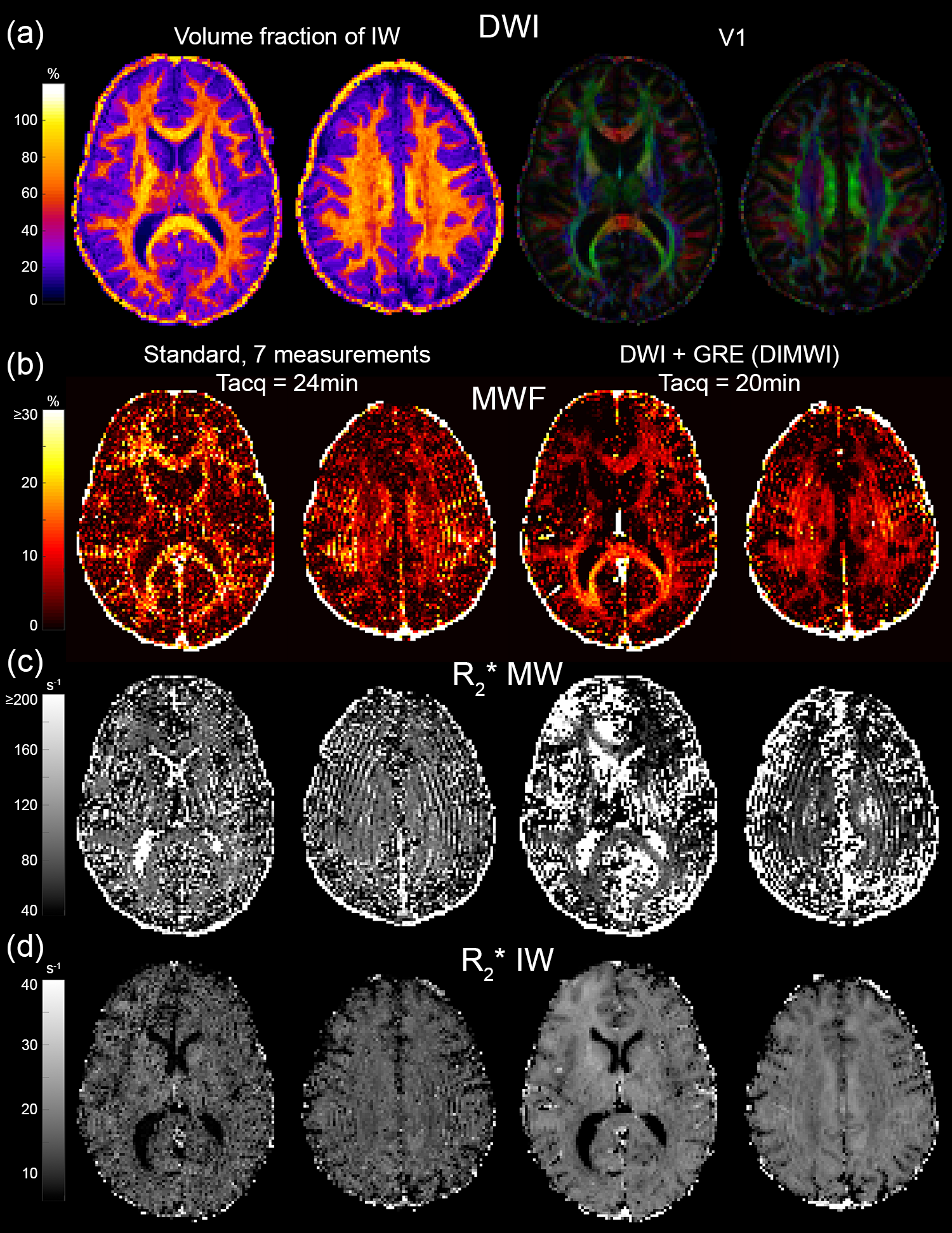
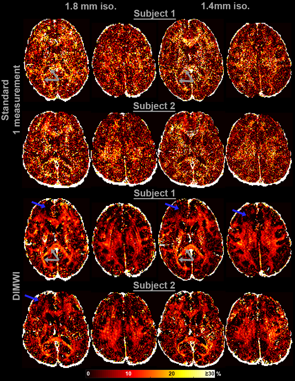
The MWF and the IW $$$R_{2}^{*}$$$ maps obtained with the standard model are significantly noisier than those of our proposed method. Fig.3 shows that even with averaging 7 GRE acquisitions, the standard model underperforms to one GRE acquisition as input to the DIMWI. Fig.4 shows that high-quality, high-resolution MWF map can be obtained with DIMWI model.

The group-averaged histograms illustrate that the MWF estimation is robust in WM (Fig.5a). Despite the DIMWI having used 3 fibre orientations from the ball-and-stick model which should account for quasi-random GM microstructure, the estimations of MWF (Fig.5b) and MW $$$R_{2}^{*}$$$ from the DIMWI (Fig.3c and Fig.5c) suggest that the biophysical model does not hold in GM. The IW $$$R_{2}^{*}$$$ of DIMWI has a narrower distribution (Fig.3d and Fig.5d), suggesting a more robust fitting, and higher values than the standard MWI (due to over-fitting).

Conclusion

Incorporating DWI into MWI improves MWF estimation in WM, allowing higher resolution MWF maps to be acquired in a shorter amount of time. DIMWI is an interesting add-on to diffusion-weighted imaging. A relatively short acquisition (3.5 minutes added to a 15-minute DWI scan) can provide information on myelin integrity that is not directly accessible using DWI. DIMWI will be combined with multi-compartment relaxometry⁷ to explore other myelination markers associated with longitudinal relaxation.

Acknowledgements

This work is part of the research programme with project number FOM-N-31/16PR1056/RadboudUniversity, which is financed by the Netherlands Organisation for Scientific Research (NWO).