Introduction

Vascular compliance (VC) represents the ability of a vessel to dilate in response to pressure alterations [1], and is an important predictor of cardiovascular disease and stroke [2,3]. While VC in other body parts can be measured with ultrasound [4], it is challenging to measure VC in intracranial vessels because of the skull [5,6]. Here, we combined ASL-based MRA with radial acquisition and compressed sensing to resolve vessel-size fluctuations across cardiac cycle with whole-intracranial-artery coverage and high resolution, from which VC was estimated.

Methods

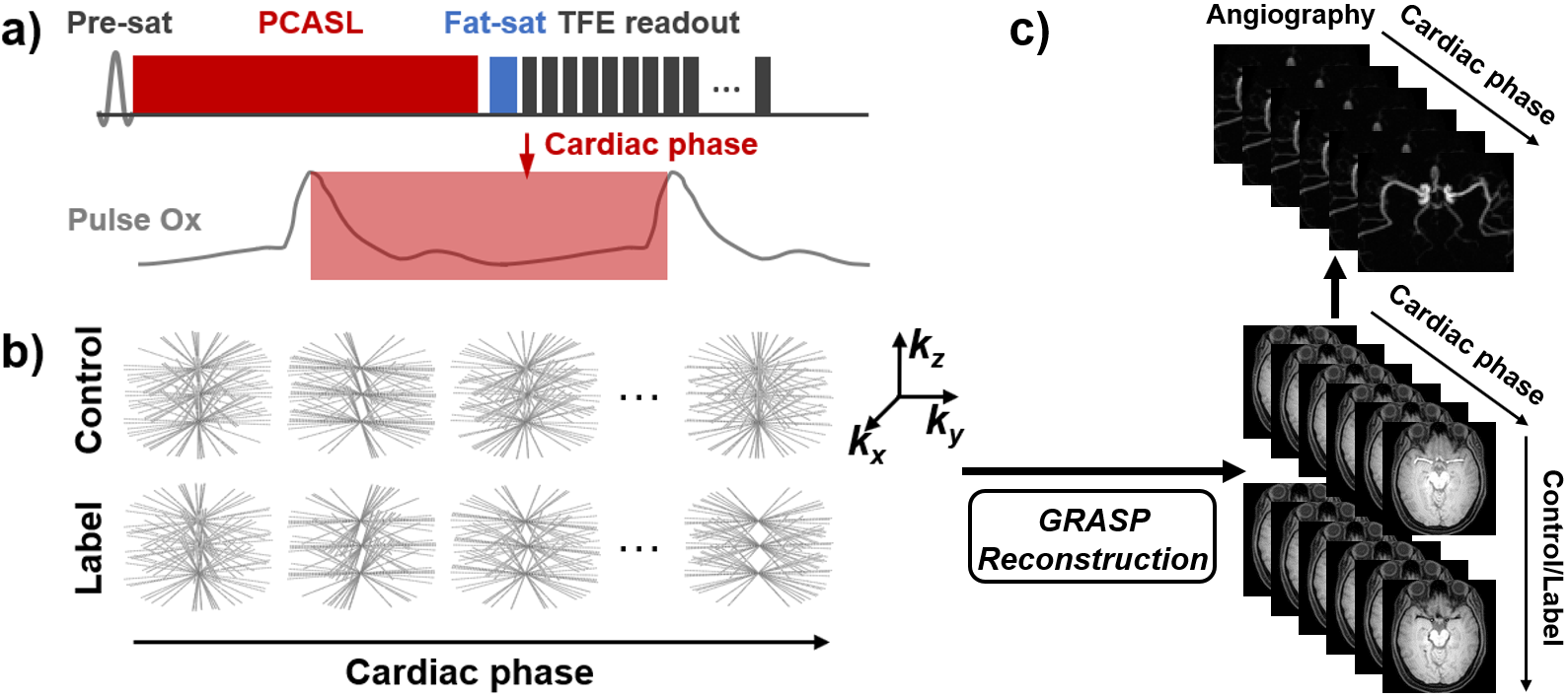
Pulse sequence: We used ASL-based MRA without post labeling delay (Fig. 1a). A stack-of-stars k-space trajectory was used, where Cartesian sampling is used along the kz direction and golden-angle radial sampling is used in the kx-ky plane. Each shot acquires all the k-lines that are parallel and of the same radial angle in a low-high-frequency order. Based on the cardiac phase of each TR recorded using a pulse device, all k-space data can be retrospectively grouped into two dynamic cardiac series, one for control and the other for label condition (Fig. 1b). Note that the k trajectories in every volume are highly under-sampled and distinct between control/label pairs or cardiac phases, in which the sparsity along cardiac dimension and control/label dimension can be exploited in the compressed sensing reconstruction.
Reconstruction: A GRASP algorithm was used to reconstruct cardiac-phase specific dynamic ASL images [7]. Briefly, the reconstruction was performed by solving $$$x=argmin\big\{\|F\cdot S\cdot x-k\| _2^2+\lambda_{cardiac}\|D_{cardiac}\cdot x\|_1+\lambda_{control/label}\|D_{control/label}\cdot x\|_1\big\}$$$. Here $$$F$$$ is NUFFT operator, $$$S$$$ is the estimated multi-coil sensitivity maps, $$$x$$$ is the 5D dynamic image series with three spatial dimensions, one cardiac-phase dimension, and one label/control dimension. $$$k$$$ is the multi-coil radial k-space data sorted according to cardiac and labeling states, $$$D_{cardiac}$$$ and $$$D_{control/label}$$$ are the differences between consecutive frames along the two dimensions, respectively. $$$\lambda_{cardiac}$$$ and $$$\lambda_{control/label}$$$ are corresponding regularization weights that control the tradeoff between data fidelity and sparsity constraints. The reconstruction yields a series of control/label images at different cardiac phases, from which a cardiac-phase-resolved angiography was obtained (Fig. 1c).
Experiment: Six healthy subjects (30.2±7.6 years, 3M/3F) were scanned on a 3T scanner (Philips), after IRB-approved informed consent was obtained. The imaging parameters were: TFE readout, TFE factor=40, TR/TE=4.7/2.1ms, FOV=180×180×80mm³, voxel size=2×2×2mm³, 40 partitions along kz, 221 spokes, acquisition duration of each shot=189ms. In order to find optimal labeling duration that is long enough to allow labeled water spins to fill the whole artery tree while maintaining reasonable scan time, various labeling durations (400, 800, 1200, and 1600ms) were performed in a subset of three subjects. A pulse device was attached to the finger of the subject, yielding R-peaks that were used to calculate cardiac phase of each acquisition. Brachial pulse pressure ΔP was measured by cuff blood pressure device as a surrogate of intracranial pulse pressure.
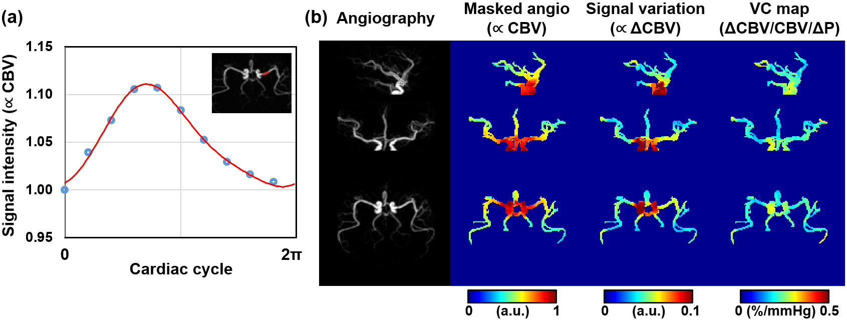
Data processing: For each voxel in the cardiac-phase-resolved angiography, its signal intensity was plotted as a function of cardiac phase and then fitted to a 2nd-order Fourier series (4 coefficients), as illustrated in Fig. 2a. The difference between upper and lower peaks is considered ΔCBV between systolic and diastolic phases. The average of the curve is proportional to baseline CBV. Therefore, voxel-by-voxel VC can be calculated accordingly by ΔCBV/CBV/ΔP.

Results

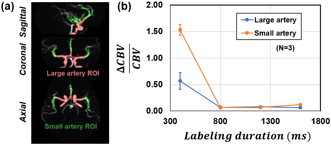
Fig. 2a shows representative CBV fluctuations as a function of cardiac phase in an ROI on MCA, which exhibits clear pulsatile modulation. Fig. 2b displays the averaged angiography across cardiac phases, signal fluctuation map, and derived VC map, respectively. Note that the signal intensities of both averaged angiography and signal fluctuation map depend on arterial arrival time due to T1 recovery of labeled blood, but their ratio, ΔCBV/CBV, is independent of arterial arrival time effect. It should also be pointed out that both ΔCBV and CBV maps show higher values in larger vessels (red), but their effects are canceled out in the VC map (far right in Fig. 2b).
Fig. 3b shows the ΔCBV/CBV dependence on labeling duration. The ΔCBV/CBV is overestimated for 400ms labeling duration in both large and small artery ROIs (Fig. 3a), due to “flow” pulsation between systolic and diastolic phases (note: we only want to measure the effect of “volume” pulsation in VC). The overestimation is more pronounced in small artery because of its longer bolus arrival time and thus more severe flow-related signal change across cardiac cycle. ΔCBV/CBV value plateaued after 800 ms, suggesting that the artery tree is filled with labeled water spins regardless of systole/diastole. This finding is consistent with artery transit time in the literature [8].
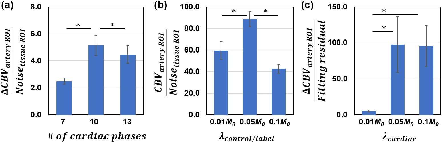
We also examined the performance of the technique on reconstruction parameters, specifically the number of cardiac phases, and the two regularization weights, $$$\lambda_{cardiac}$$$ and $$$\lambda_{control/label}$$$ (Fig. 4). It was found that 10 cardiac phases with $$$\lambda_{control/label}$$$=0.05 and $$$\lambda_{cardiac}$$$=0.05 provides the best SNR.
Fig. 5 exhibits an animation of pulsatile angiography and the corresponding VC map (click the multi-media file to see animations).

Conclusion

We proposed a technique to map vascular compliance along the entire intracranial arterial tree. This method may have potential utility in studies of cerebral arteriosclerosis, hypertension, diabetes, and related diseases.

Acknowledgements

None.