Introduction

The physics principle governing the passage of tracer in tissue is the transport equation of mass flux¹. This transport equation description of perfusion precludes the notion of arterial input function (AIF)². The inverse problem of the transport equation has recently been considered for mapping the 3D velocity field of water transit in tissue from multi-delay 3D arterial spin labeling MRI data^2,3, and is termed as QTM. Solving the inverse problem requires voxelization of the continuous transport equation based on the vasculature inside the voxel. Here we report QTM in brain tumor, where the vasculature is approximated as a porous medium⁴, and QTM leads to mapping of the voxel-averaged tracer velocity. The porous medium approximation is validated using rigorous solutions of the transport equations in numerical phantoms using finite element modeling. QTM is applied to dynamic contrast enhanced (DCE) MRI data, and the QTM velocity field was compared with the flow map obtained using the traditional Kety’s method.

Methods

Porous media QTM Algorithm:
Voxelized transport equation in the porous media approximation is⁴: $$\partial_{t}c\left(\boldsymbol{\xi},t\right)=-\nabla\cdot c\left(\boldsymbol{\xi},t\right)\boldsymbol{u}\left(\boldsymbol{\xi}\right)+\nabla\cdot\tau\left(\boldsymbol{\xi}\right)\nabla c\left(\boldsymbol{\xi},t\right)$$ Here $$$c\left(\boldsymbol{\xi},t\right)$$$ is the tracer concentration averaged over voxel $$$\boldsymbol{\xi}$$$, $$$u\left(\boldsymbol{\xi}\right)=\left[u^{x},u^{y},u^{z}\right]$$$ the averaged velocity, $$$\tau\left(\boldsymbol{\xi}\right)$$$ the pseudo-tortuosity coefficient representing the porous tortuosity and diffusion effects averaged over the voxel at $$$\boldsymbol{\xi}$$$. Let $$$u\left(\boldsymbol{\xi}\right)=[u^x(\boldsymbol{\xi}),u^y(\boldsymbol{\xi}),u^z(\boldsymbol{\xi}),\tau(\boldsymbol{\xi})]\equiv[\boldsymbol{u},\tau]$$$, and organize the discretized Eq.1 at all voxels in an imaging volume as $$$A\overrightarrow{u}=\overrightarrow{b}$$$, where $$$A$$$ is a sparse matrix containing divergence operator and $$$\nabla c(\boldsymbol{\xi},t_i)$$$, $$$\overrightarrow{u}$$$ and $$$\overrightarrow{b}$$$ vector obtained by concatenating $$$u\left(\boldsymbol{\xi}\right)$$$ and $$$\partial_{t}c\left(\boldsymbol{\xi},t\right)$$$ of all voxels, respectively. The inverse problem reconstructing velocity field and pseudo-tortuosity is formulated as a constrained minimization problem: $$\overrightarrow{u}=argmin_{\overrightarrow{u}}\left\Vert A\overrightarrow{u}-\overrightarrow{b}\right\Vert _{2}^{2}+\lambda\left\Vert \nabla\overrightarrow{u}\right\Vert ^{2}$$ An L2 regularization is added in Eq.2 for denoising with $$$\lambda=10^{-3}$$$ chosen empirically according to minimal mean square error with respect to the ground truth in simulation and in vivo image quality and L-curve characteristics.
Numerical validation:
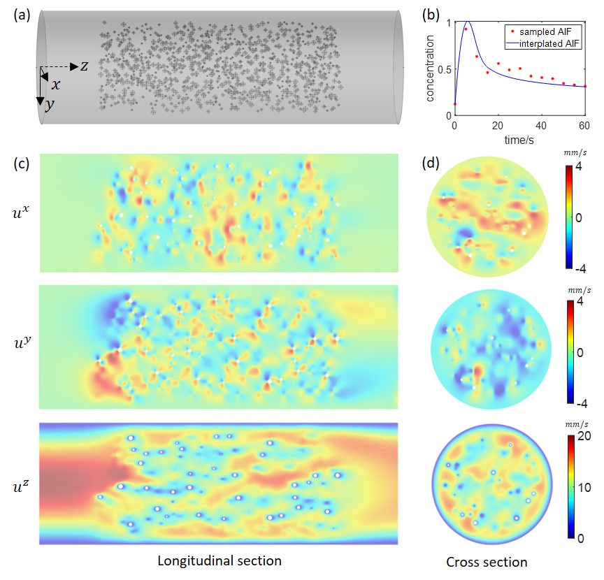
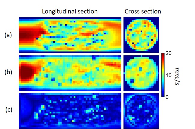
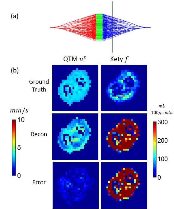
We first generated a numerical phantom consisting of a cylindrical volume (radius 1cm and length 6 cm) filled with randomly placed solid spheres (Fig.1a). The continuous media Navier-Stokes equation was solved using a finite element method (FEM) with an inlet boundary condition of parabolic flow with a maximum velocity of 2cm/s, and an outlet boundary condition of zero pressure. To simulate a 4D tracer concentration image data, the continuity equation was solved with a 0.05s time interval for 100s using FEM and a concentration time curve at the inlet being that of a feeding artery of a brain tumor measured in one of the patients. Next, we generated a vessel tree network by a random branching rule⁵ in a double-cone shape of similar size and flow (Fig.3a). The ground truth consisted of the simulated velocity map at imaging resolution (Figs.2a&3b_top_left) and flow (Fig.3b_top_right). The simulated concentration data was then down-sampled to spatiotemporal resolution of imaging data (1x1x1 mm³ voxel size and 5s temporal frame) as an input of QTM reconstruction.
In vivo DCE MRI
10 brain tumors were acquired using a T1-weighted 3D MRI sequence before and after the injection of gadolinium contrast agent using the following parameters: 0.94x0.94x5 mm³ voxel size, 256x256x(16-34) matrix size, 13-25° flip angle, 1.21-1.35 ms TE, 4.37-5.82 ms TR, 6.2-10.2 s temporal resolution, and 30-40 time points. QTM processing by Eq.2 was performed on all data. The DCE image data was converted to gadolinium concentration ([Gd]) data by assuming a linear relationship between signal intensity change and contrast agent concentration⁶. The velocity amplitude of each voxel was calculated as follows: $$\left|\boldsymbol{u}\left(\boldsymbol{\xi}\right)\right|=\sqrt{\left(u^{x}\left(\boldsymbol{\xi}\right)\right)^{2}+\left(u^{y}\left(\boldsymbol{\xi}\right)\right)^{2}+\left(u^{z}\left(\boldsymbol{\xi}\right)\right)^{2}}$$ For comparison, traditional Kety’s regional blood flow ($$$f_{kety}$$$) maps (ml/100g/min) were also obtained: $$\partial_{t}c\left(\boldsymbol{\xi},t\right)=f_{kety}\left(\boldsymbol{\xi}\right)\left[c_{A}(t)-c\left(\boldsymbol{\xi},t\right)/v(\boldsymbol{\xi})\right]$$ where $$$c_A(t)$$$ was the global arterial input function (AIF) and $$$v(\boldsymbol{\xi})$$$ the regional blood volume and data fitting to Eq.4 included AIF delay adjustment (19).

Results

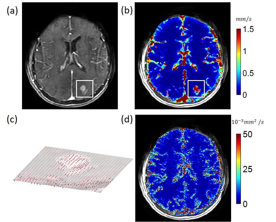
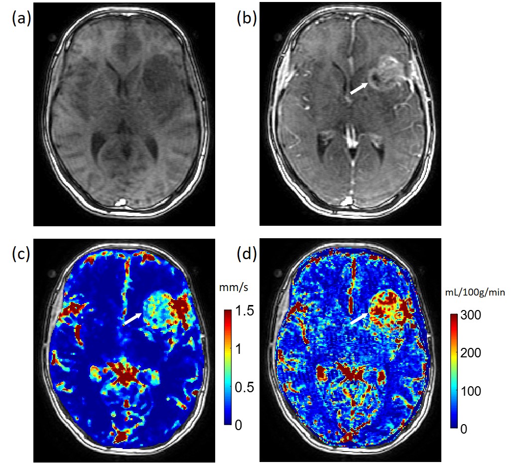
In the simulation of random spherical inclusions, QTM method successfully reconstructed velocity field with high correlation with the ground truth and negligible bias (Fig.2), resulting in a linear regression of slope=1.02, R² = 0.89. The estimated pseudo tortuosity values varied from $$$ 5 to 50\times10^{-3}$$$ mm³/s inside phantom, which bore little correlation with the ground truth diffusion coefficient (slope=$$$5\times 10^{-10}$$$, R² =0.2). In the simulation of random-branching vasculature, QTM showed higher concordance with the ground truth (slope=1.01, R² = 0.82), while Kety’s method showed overestimation in the second half of the phantom (slope=8.3, R² = 0.27).
For in vivo DCE MRI, QTM automatedly processed all data while Kety’s method required manual AIF input. Fig.4 exemplifies velocity magnitude, velocity vector and tortuosity map of a glioblastoma. Fig.5 exemplified comparison of QTM $$$|\boldsymbol{u}|$$$ and $$$f_{Kety}$$$: a region of low enhancement showed low $$$|\boldsymbol{u}|$$$ but high $$$f_{Kety}$$$.

Discussion and Conclusion

In simulations with known ground truths, QTM mapped velocity field with good accuracy as demonstrated in phantoms with spherical inclusions and with a vascular network. On the other hand, Kety’s method suffered large errors. For all brain tumor DCE MRI data, QTM velocity maps were automatically generated, while Kety’s method required a manual selection of arterial input function. Distinct flow pattern in the tumor was observed between two methods. Automated QTM for characterizing transport velocity is feasible by inverting an apparent voxelized equation of mass flux in porous tissue model for tumor DCE MRI data.

References

1.Landau LD, Lifshit︠s︡ EM. Fluid mechanics. Oxford, England; New York: Pergamon Press; 1987. xiii, 539 p., 531 leaf of plates p.
2. Spincemaille P, Zhang Q, Nguyen TD, Wang Y. Vector field perfusion imaging. ISMRM, 2017; Hawaii. p 3793.
3. Zhou L, Zhang Q, Spincemaille P, Nguyen T, Wang Y. Quantitative Transport Mapping (QTM) of the Kidney using a Microvascular Network Approximation. ISMRM, 2019; Montreal. p 703.
4. Bear J. Dynamics of fluids in porous media: Courier Corporation; 2013 5. Schabel MC, Parker DL. Uncertainty and bias in contrast concentration measurements using spoiled gradient echo pulse sequences. Phys Med Biol 2008;53(9):2345-2373.