0005

Multiphoton Magnetic Resonance Imaging

Victor Han¹ and Chunlei Liu^1,2
¹Electrical Engineering and Computer Sciences, University of California, Berkeley, Berkeley, CA, United States, ²Helen Wills Neuroscience Institute, University of California, Berkeley, Berkeley, CA, United States

Synopsis

We present a fully geometric view of multiphoton excitation by taking a particular rotating frame transformation. In this rotating frame, we find that multiphoton excitations appear just like single-photon excitations again, and thus, we can readily generalize concepts already explored in standard single-photon excitation. With a homebuilt low-frequency (~ kHz) coil, we execute a standard slice-selective pulse sequence with all of its excitations replaced by their equivalent two-photon versions. With a multiphoton interpretation of oscillating gradients, we present a novel way to transform a standard slice-selective adiabatic pulse into a multiband one without modifying the RF pulse shape itself.

Introduction

Today’s MRI assumes single-photon excitation¹. That is, for each nuclear spin, a single photon accompanies the transition between energy states. This photon must resonate near the Larmor frequency. Here, we show that, instead of the usual single-photon resonance, we can excite multiphoton resonances to generate signal for MRI by using multiple magnetic field frequencies, none of which is near the Larmor frequency. Only the total energy absorbed by a spin must correspond to the Larmor frequency. Multiphoton excitation has been described for NMR^2–5 and EPR^6,7. For MRI, however, multiphoton excitation has not yet been well explored. The idea that oscillating z-direction magnetic fields creates frequency “sidebands” is well known and has been used occasionally, both in excitation⁸ and reception⁹. For excitation, it was used for simultaneous transmit and receive, and for reception, it was used to accelerate spatial information acquisition by increasing the receive bandwidth. However, as we will show, a multiphoton framework paints a more complete picture than sideband excitation, and with it, we are able to better understand some of the subtleties involved. Within this framework, it becomes clear that these multiphoton excitations excite extra resonances, and concepts such slice selective excitation and adiabatic RF pulses readily generalize.

Theory

Standard single-photon excitation occurs when the RF field is polarized in the xy-plane ($$$B_{1,xy}$$$), perpendicular to the main magnetic field $$$B_0$$$. Multiphoton effects occur when we add more RF fields along the z-axis ($$$B_{1,z}$$$), parallel to the main magnetic field $$$B_0$$$. The term RF is used very loosely to include any oscillation frequency. Although it is also possible to have multiphoton effects with RF only in the xy-plane⁵, the effects are usually orders of magnitude smaller.

To analyze multiphoton excitation, consider two $$$B_1$$$ fields with frequencies $$$\omega_{xy}$$$ and $$$\omega_z$$$ along the xy-plane and z-axis respectively. The total magnetic field in the laboratory frame is $$B_z=B_0+B_{1,z}\cos{\left(\omega_zt\right)}\hspace{2em}[1]$$ $$B_x=B_{1,xy}\cos{\left(\omega_{xy}t\right)}\hspace{2em}[2]$$ $$B_y=-B_{1,xy}\sin{\left(\omega_{xy}t\right)}\hspace{2em}[3]$$ where the RF field in the xy-plane is clockwise circularly polarized; $$$B_{1,xy}$$$ and $$$B_{1,z}$$$ are amplitudes of each RF field. In a clockwise rotating frame with an angular velocity of $$$\omega_{rot}$$$, the effective $$$B_z$$$ field is $$B_{z,eff}=B_z-\frac{\omega_{rot}}{\gamma}\hspace{2em}[4]$$ To generate time-invariant $$$B_{z,eff}$$$, we choose $$\omega_{rot}=\omega_{xy}+\gamma B_{1,z}\cos{\left(\omega_zt\right)}\hspace{2em}[5]$$ We refer to this rotating frame as the phase-modulated rotating frame followingMichal². This choice of $$$\omega_{rot}$$$ results in a non-stationary xy-plane RF field. To illustrate this effect, we examine the phase accrual of the xy-RF field in the rotating frame. Let $$$\theta$$$ be the phase, then $$B_{x,eff}=B_{1,xy}\cos{\left(\theta\right)}\hspace{2em}[6]$$ $$B_{y,eff}=B_{1,xy}\sin{\left(\theta\right)}\hspace{2em}[7]$$ By definition, $$\theta=\int_{0}^{t}{(\omega_{rot}}-\omega_{xy})dt=\frac{\gamma B_{1,z}}{\omega_z}\sin{\left(\omega_zt\right)}\hspace{2em}[8]$$ Combining Eqs. [4-8] gives $$B_{z,eff}=B_0-\frac{\omega_{xy}}{\gamma}\hspace{2em}[9]$$ $$B_{x,eff}=B_{1,xy}\cos{\left(\frac{\gamma B_{1,z}}{\omega_z}\sin{\left(\omega_zt\right)}\right)}\hspace{2em}[10]$$ $$B_{y,eff}=B_{1,xy}\sin{\left(\frac{\gamma B_{1,z}}{\omega_z}\sin{\left(\omega_zt\right)}\right)}\hspace{2em}[11]$$ Eqs. [10,11] can be Taylor expanded if $$$\frac{\gamma B_{1,z}}{\omega_z}\ll1$$$ as $$B_{x,eff}\approx B_{1,xy}\hspace{2em}[12]$$ $$B_{y,eff}\approx B_{1,xy}\frac{\gamma B_{1,z}}{\omega_z}\sin{\left(\omega_zt\right)}\hspace{2em}[13]$$ From Eqs. [9,12,13], three potential resonances exist depending on the relative values of the frequencies (Fig. 1).

Single-photon resonance: If $$$\omega_{xy}=\gamma B_0$$$, then $$$B_{z,eff}=0$$$ and $$$B_{x,eff}$$$ tilts magnetization from the z-axis. This is the normal on-resonance condition.
Two-photon resonances: If $$$\omega_{xy}=\gamma B_0\pm\omega_z$$$, then $$$B_{z,eff}=\mp\frac{\omega_z}{\gamma}$$$. The linearly polarized RF field $$$B_{y,eff}$$$ oscillates with an angular frequency of $$$\omega_z$$$, matching the amplitude of $$$B_{z,eff}$$$, which induces resonances. These two new resonances correspond to state transitions where a single xy-polarized photon is absorbed and a single z-polarized photon is absorbed or emitted, depending on whether the xy-frequency is below or above the Larmor frequency. From Eq. [13], consistent with past work, the effective angular nutation frequency for two-photon excitation is $$\omega_{nut}=\frac{\gamma B_{1,xy}\gamma B_{1,z}}{2\omega_z}\hspace{2em}[14]$$ If more terms are kept in the Taylor expansion of Eqs. [10,11], we can analyze higher-order excitations with three or more photons. However, Taylor expansion requires $$$\frac{\gamma B_{1,z}}{\omega_z}\ll1$$$. Alternatively, we can exactly expand $$$B_{x,eff}$$$ and $$$B_{y,eff}$$$ using Bessel functions, which reveals that for any integer $$$n$$$, resonance occurs whenever $$\omega_{xy}=\gamma B_0+n\omega_z\hspace{2em}[15]$$ and for each integer $$$n$$$, the corresponding effective angular nutation frequency is $$\omega_{nut}=\gamma B_{1,xy}J_n\left(\frac{\gamma B_{1,z}}{\omega_z}\right)\hspace{2em}[16]$$

Methods

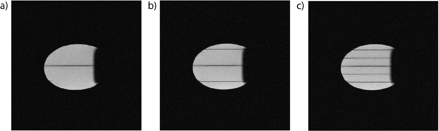
Multiphoton resonances were verified in simulation. With an extra solenoid coil in the $$$B_0$$$ direction, images of a lemon and pork rib were acquired with all standard excitations replaced by effectively equivalent two-photon versions (setup in Fig. 2). Without extra hardware, a vendor provided adiabatic inversion pulse was played out with superimposed oscillating and constant gradients to produce a multiband version. All experiments were on an Aspect 1T wrist scanner (Aspect Imaging, Shoham, Israel).

Results

Fig. 3 shows simulated lines depicting multiphoton resonances, Fig. 4 shows single- and two-photon images of a lemon and pork rib, and Fig. 5 shows a multiband inversion.

Discussion and Conclusions

In the phase-modulated rotating frame, we see that multiphoton excitation looks just like a scaled single-photon excitation with some extra off-resonant fields. As shown here, with a constant amplitude $$$B_{1,z}$$$ field, frequency-offset slice selective $$$B_{1,xy}$$$ fields act as scaled versions of their single photon counterparts, whether they are adiabatic or not. Multiphoton excitation provides insight for designing excitation pulses, with or without extra hardware, and can potentially be used for spin-locking experiments to explore novel contrast for MRI with z-axis frequencies chosen to probe biological or chemical processes of interest. As gradient^10,11 and traditional RF coils gain more channels and spatial-temporal flexibility, much more can be achieved using multiphoton MRI to encode spatial, spectral and temporal information.

Acknowledgements

The authors thank Michael Lustig, PhD, of UC Berkeley for discussions and assistance with the Aspect scanner, Neelesh Ramachandran of UC Berkeley for assistance with hardware construction, and Aspect Imaging for providing the scanner.

References

1. Lauterbur PC. Image Formation by Induced Local Interactions: Examples Employing Nuclear Magnetic Resonance. Nature. 1973;242(5394):190-191. doi:10.1038/242190a0

2. Michal CA. Nuclear magnetic resonance noise spectroscopy using two-photon excitation. The Journal of Chemical Physics. 2003;118(8):3451-3454. doi:10.1063/1.1553758

3. Eles PT, Michal CA. Two-photon two-color nuclear magnetic resonance. The Journal of Chemical Physics. 2004;121(20):10167-10173. doi:10.1063/1.1808697

4. Eles PT, Michal CA. Two-photon excitation in nuclear magnetic and quadrupole resonance. Progress in Nuclear Magnetic Resonance Spectroscopy. 2010;56(3):232-246. doi:10.1016/j.pnmrs.2009.12.002

5. Zur Y, Levitt MH, Vega S. Multiphoton NMR spectroscopy on a spin system with I =1/2. The Journal of Chemical Physics. 1983;78(9):5293-5310. doi:10.1063/1.445483

6. Gromov, Schweiger. Multiphoton resonances in pulse EPR. Journal of magnetic resonance. 2000;146(1):110-121. doi:10.1006/jmre.2000.2143

7. Saiko AP, Fedaruk R, Markevich SA. Multi-photon transitions and Rabi resonance in continuous wave EPR. Journal of Magnetic Resonance. 2015;259:47-55. doi:10.1016/j.jmr.2015.07.013

8. Brunner D, Pavan M, Dietrich B, Rothmund D, Heller A, Pruessmann K. Sideband Excitation for Concurrent RF Transmission and Reception. In: ISMRM Annual Scientific Meeting & Exhibition. Montreal, Quebec, Canada; 2011.

9. Scheffler K, Loktyushin A, Bause J, Aghaeifar A, Steffen T, Schölkopf B. Spread-spectrum magnetic resonance imaging. Magnetic Resonance in Medicine. 2019;82(3):877-885. doi:10.1002/mrm.27766

10. Littin S, Jia F, Layton KJ, et al. Development and implementation of an 84-channel matrix gradient coil. Magnetic Resonance in Medicine. 2018;79(2):1181-1191. doi:10.1002/mrm.26700

11. Ertan K, Taraghinia S, Sadeghi A, Atalar E. A z-gradient array for simultaneous multi-slice excitation with a single-band RF pulse. Magnetic Resonance in Medicine. 2018;80(1):400-412. doi:10.1002/mrm.27031

Figures

Fig. 1 – Single- and two-photon excitation conditions. a) Magnetic field setup with xy- and z-RF fields. b) In the phase-modulated rotating frame with $$$\omega_{xy}=\gamma B_0-\omega_z$$$, there is a static z-field that resonates with the oscillating field on the y-axis. Here, both a xy- and z-photon are absorbed. c) When $$$\omega_{xy}=\gamma B_0$$$, there is no z-field, and the static x-field causes a normal resonance. d) When $$$\omega_{xy}=\gamma B_0+\omega_z$$$, there is a z-field that resonates with the oscillating field on the y-axis. Here, we absorb and emit.

Fig. 2 – Example two-photon scanning setup. An extra $$$B_{1,z}$$$ solenoid is aligned with $$$B_0$$$. The control signal for the transmit/receive-switch (T/R switch) from the scanner triggers output from the waveform generator. The triggered 130 kHz signal is amplified and fed into the $$$B_{1,z}$$$ coil.

Fig. 3 – Multiphoton resonance. a) Transverse magnetization vs. 2D frequency sweep with xy-frequencies relative to Larmor and 10 ms hard pulses. One, two and three photon resonance lines can be seen. For each simulated point, $$$B_{1,z}$$$ was chosen such that $$$\frac{\gamma B_{1,z}}{\omega_z}=1$$$. $$$B_{1,xy}$$$ was a constant $$$1$$$ $$$\mu$$$T. b) Example time domain fields for the $$$B_1$$$ pulses generating a two-photon resonance and c) the corresponding frequency-domain fields. The three curves overlap in (c). There is no Larmor frequency component.

Fig. 4 – Two-photon gradient-echo sequence. a) Single-photon excitation for a lemon. b) Two-photon excitation for the lemon. c) Single-photon excitation for a pork rib. d) Two-photon excitation for the pork rib. In (b) and (d), all transmit xy-RF was shifted up by 130 kHz and a 130-kHz square wave z-RF was transmitted simultaneously with the xy-RF. TR/TE = 500/3.0 ms, FA = 10°, 500-µs sincgauss pulse for the lemons, and TR/TE = 500/8.4 ms, FA = 45°, 10-ms sincgauss pulse for the pork.

Fig. 5 – Multiband multiphoton adiabatic inversion. Inversion bands were imaged with an inversion pulse slice selection in the readout direction and a delay. a) Single-band inversion using a standard hyperbolic secant and a constant gradient pulse. b) Three-band inversion with the same hyperbolic secant pulse and a constant plus oscillating gradient pulse. c) Five-band inversion with the same hyperbolic secant pulse and a constant plus oscillating gradient at half the frequency of that in (b).

Proc. Intl. Soc. Mag. Reson. Med. 28 (2020)

0005