ASL: Analysis
1University of Manchester, United Kingdom
Synopsis
ASL acquisition produces perfusion-weighted images through the subtraction of label and control images. These may be collected at a single post-labelling delay time or at multiple delay times. How do we extract quantitative CBF from these subtraction images? Quantification is important as the signal in the perfusion-weighted images will be affected by parameters other than blood flow, principally arterial transit time, labelling efficiency and the T1 and equilibrium magnetisation of blood. These may vary on an individual and/or regional basis. In this talk I will describe the most widely used method for quantification (Alsop et. al. 2015) and explain which parameters are most important for CBF accuracy.
TARGET AUDIENCE
Clinicians and scientists new to ASLOUTCOME/OBJECTIVES
Understand how to extract cerebral blood flow (CBF) estimates from ASL data and how acquisition and analysis choices may limit the accuracy of the CBF estimate.PURPOSE
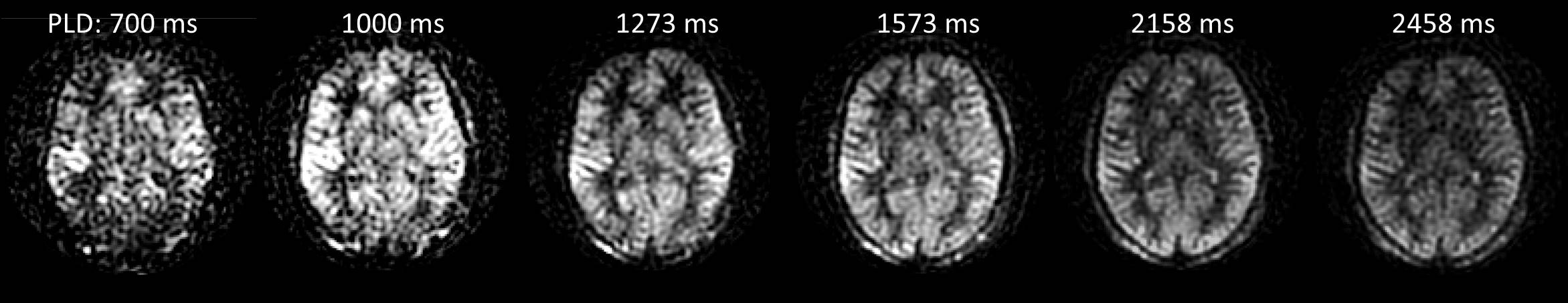
ASL acquisition produces perfusion-weighted images through the subtraction of label and control images. These may be collected at a single post-labelling delay time or at multiple delay times (Figure 1). How do we extract quantitative CBF from these subtraction images? Quantification is important as the signal in the perfusion-weighted images will be affected by parameters other than blood flow, principally arterial transit time (from the labelling plane to the tissue voxel), labelling efficiency and the T1 and equilibrium magnetisation of blood. These may vary on an individual and/or regional basis. In this talk I will describe the most widely used method for quantification (Alsop et. al. 2015) and explain which parameters are most important for CBF accuracy.SINGLE COMPARTMENT MODEL FOR THE ESTIMATION OF CBF
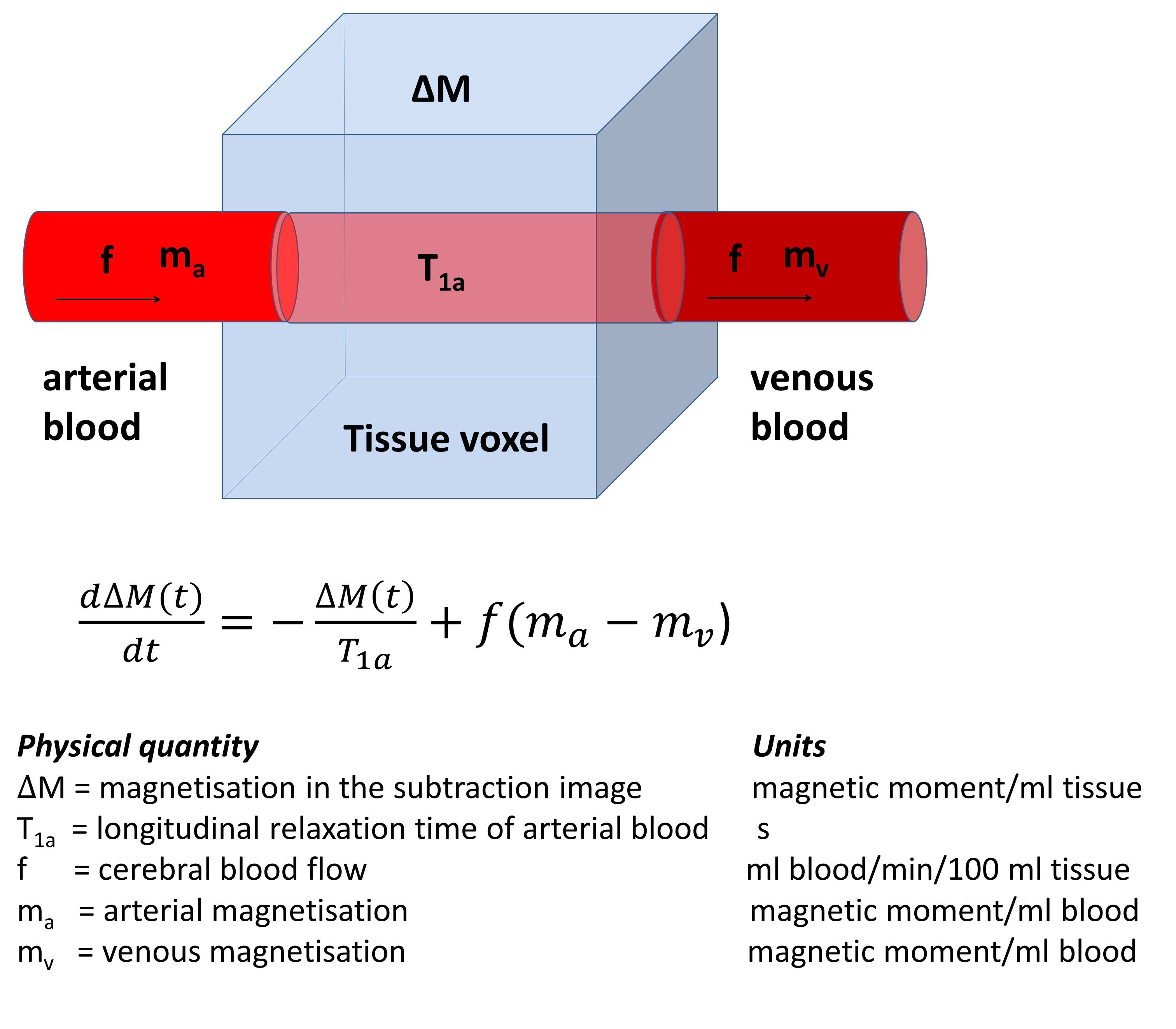
The signal
in the subtraction image is proportional to the tissue magnetisation ΔM(t)
which increases as labelled spins enter the voxel via the arterial blood and decreases
as spins leave via the venous blood and is modulated by T1
relaxation (Figure 2). The time
evolution of ΔM(t) at post-label delay time t (i.e. the end of the labelling pulse is at t=0) can be described by equation
[1] where f is
cerebral blood flow, T1a is the arterial relaxation of arterial
blood, ma is the arterial magnetisation and mv is the
venous magnetisation. The widely accepted standard approach for modelling the
ASL signal (Alsop et. al. 2015) is to make the following assumptions:
1. The relaxation of labelled spins is governed by the T1 of arterial
blood.
This is implicit in equation [1] and assumes that the labelled spins do not
exchange with the tissue spins during the post-labelling delay time. This
assumption is not true as water will exchange across the capillary wall however
the error to the CBF estimate is generally relatively small. Note that the
error may be larger in white matter where the difference in T1
between blood and tissue is larger and in applications outside the brain where
exchange of water may be greater.
2. There is no outflow of labelled blood water (the venous magnetisation mv
= 0)
This is generally true because (i) it takes several seconds for blood to transit
through the capillary bed so little perfusing labelled blood leaves the voxel
during the post-labelling delay time and (ii) most of the labelled water is
extracted from the blood into the tissue. In addition, if any labelled blood
water does leave the voxel in the venous blood it will carry very little
magnetisation as this will have largely decayed due to T1
relaxation. Any error that this assumption introduces into the CBF estimation
will be very small.
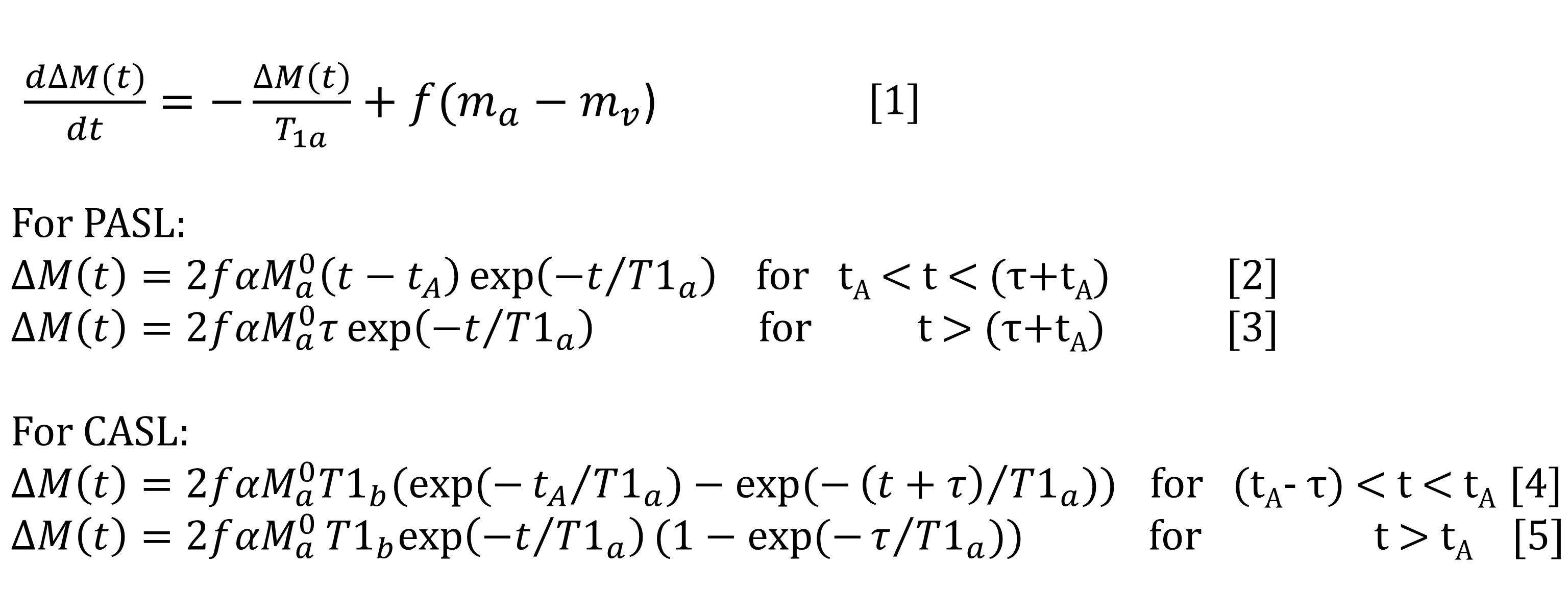
These
assumptions allow a relatively simple solution to equation [1] as derived by
Buxton et. al. (1998) and Parkes et. al. (2002) and as suggested in the recent
consensus paper (Alsop et al 2015). Equations [2-5] show these solutions where α is the labelling efficiency, Ma0
is the equilibrium magnetisation of arterial blood, tA is the
arterial transit time, τ is the duration (or temporal width) of the labelled bolus
and t is the post-labelling delay time (often referred to as the inversion time
for PASL). QUIPSS II (Wong et. al. 1998) provides an important modification to
PASL acquisition schemes, allowing the bolus duration τ to be prescribed as the
acquisition parameter TI1. For CASL acquisition schemes, τ is
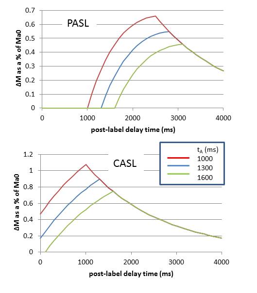
prescribed as the labelling duration. Figure 3 shows the form of equations [2-5]
for a range of arterial transit times.
SINGLE vs MULTIPLE POST-LABELLING DELAY TIMES
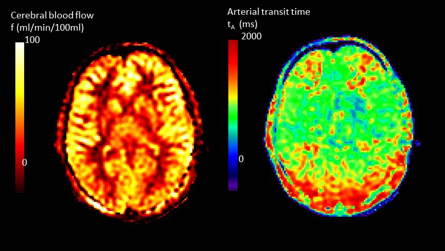
If acquisition is at a single post-labelling delay time then it is important that this time is chosen to be greater than the arterial transit time (tA). Only then will the signal be insensitive to this delay time (Figure 3). However, in striving to avoid transit time effects, the post-labelling delay time may be chosen to be longer than strictly necessary, compromising signal to noise ratio. A multi-time point measure allows both CBF and tA to be estimated by fitting the solution for ∆M(t) to the data using equations [2-5]. Figure 4 shows maps of CBF and tA acquired by fitting equations [4] and [5] to the data shown in Figure 1. It can be seen that tA has some regional differences being longer at the boundaries of the vascular territories. If arterial arrival time is not corrected for, this may introduce errors in the regional pattern of CBF. It is particularly important to correct for arterial transit time in clinical applications where arrival time may be longer than expected due to collateral circulation or slower flow velocities. In addition, there is increasing interest in the arrival time itself, as it may reflect important aspects of the underlying physiology.FACTORS AFFECTING ACCURACY OF CBF
As evident from the kinetic model described above, accurate quantification of CBF requires knowledge of several additional parameters including longitudinal relaxation time of arterial blood (T1a), labeling efficiency (α), and the equilibrium magnetization of blood (Ma0). These parameters can be either be measured or literature values can be used. While all 3 of these parameters have a large impact on CBF, they are ‘global parameters’ that will not affect the regional perfusion patterns – only the absolute quantification.CONCLUSION
Wide consensus has now been reached regarding a pragmatic approach to quantification of CBF in the brain (Alsop et al, 2015). Ongoing work indicates the benefits of acquiring multi delay time data in terms of improved accuracy of CBF and additional metrics of clinical relevance such as arterial transit time.Acknowledgements
No acknowledgement found.References
David C. Alsop, John A. Detre, Xavier Golay, Matthias Gunther, Jeroen Hendrikse, Luis Hernandez-Garcia, Hanzhang Lu, Bradley J. MacIntosh, Laura M. Parkes, Marion Smits, Matthias J. P. van Osch, Danny JJ Wang, Eric C. Wong, Greg Zaharchuk, ‘Recommended Implementation of Arterial Spin Labeled Perfusion MRI for Clinical Applications: A consensus of the ISMRM Perfusion Study Group and the European Consortium for ASL in Dementia’ Mag Res Med 73(1):102-116 Jan [2015]. DOI: 10.1002/mrm.25197.
Buxton RB, Frank LR, Wong EC, Siewert B, Warach S, Edelman RR.A general kinetic model for quantitative perfusion imaging with arterialspin labeling. Magn Reson Med 40:383–396 [1998].
Parkes LM and Tofts PS, ‘Improved Accuracy of Human Cerebral
Blood Perfusion Measurements using Arterial Spin Labelling, Accounting for
Capillary Water Permeability’ Magnetic Resonance in Medicine 48, 27-41 July
[2002]. DOI: 10.1002/mrm.10180.
Wong EC, Buxton RB, Frank LR. Quantitative imaging of perfusionusing a single subtraction (QUIPSS and QUIPSS II). Magn Reson Med 39:702–708 [1998].
Figures