Field Probes for Characterizing & Calibrating MRI Systems
1Institute for Biomedical Engineering, University and ETH Zurich, Zurich, Switzerland, 2Skope MRT, Zurich, Switzerland
Synopsis
Driving MR image acquisitions requires a level of accuracy of the dynamics of the magnetic fields that is almost impossible to achieve by design. Induced eddy currents, lead inductances, amplifier delays and other effects have hence to be corrected by feed-back, pre-distortion and post-correction schemes. All these approaches however are based on accurate characterizations of the field evolution in the scanner. In this talk, characterization methods based on field probes will be discussed along with the application of the obtained data for system calibration.
Introduction
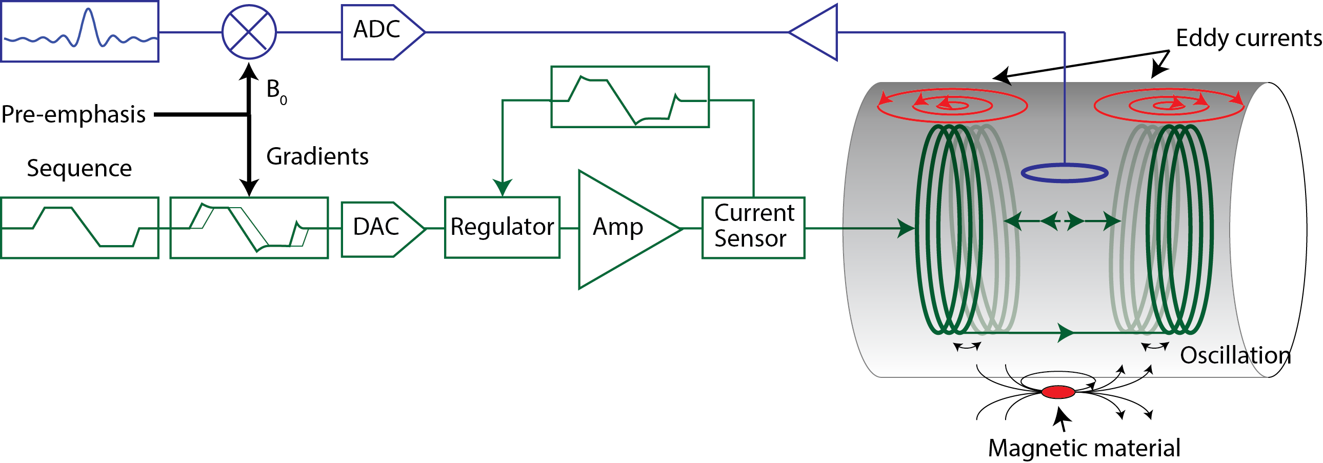
The spatial-temporal dynamics of the magnetic field inside the scanner generates and encodes the NMR signals. To correctly manipulate the spin coherences but also to interpret and reconstruct images from the acquired raw signals the evolution of the magnetic field inside the scanner has to be controlled. The employed hardware cannot natively provide the accuracy in the field dynamics that is ideally required. Image distortions resulting from spatial field non-idealties can mostly be handled in post-processing by unwarping the images to remove the geometrical distortion [1]. In turn, realizing the desired temporal evolution of the magnetic field in the scanner is more complex. Stray induction into conductive surfaces (eddy currents), mechanical interactions and externally induced fields cause delays, distortions or fluctuations that heavily impair the resulting image quality. In order to obtain the required accuracy in the field evolution, MRI scanners require therefore very accurate compensation and correction schemes in order to overcome the remnant shortcomings of the employed hardware. The basic principle behind this approach is that calibration, compensation and correction schemes (Fig.1) can turn the precision and accuracy achieved in measurements of the magnetic field evolution into an enhanced fidelity of the acquisition and reconstruction. This in turn implies that the accuracy by which the dynamic fields are measured sets the ultimate boundary for the achievable accuracy in the experiments.Measurement methods for field dynamics in MRI systems
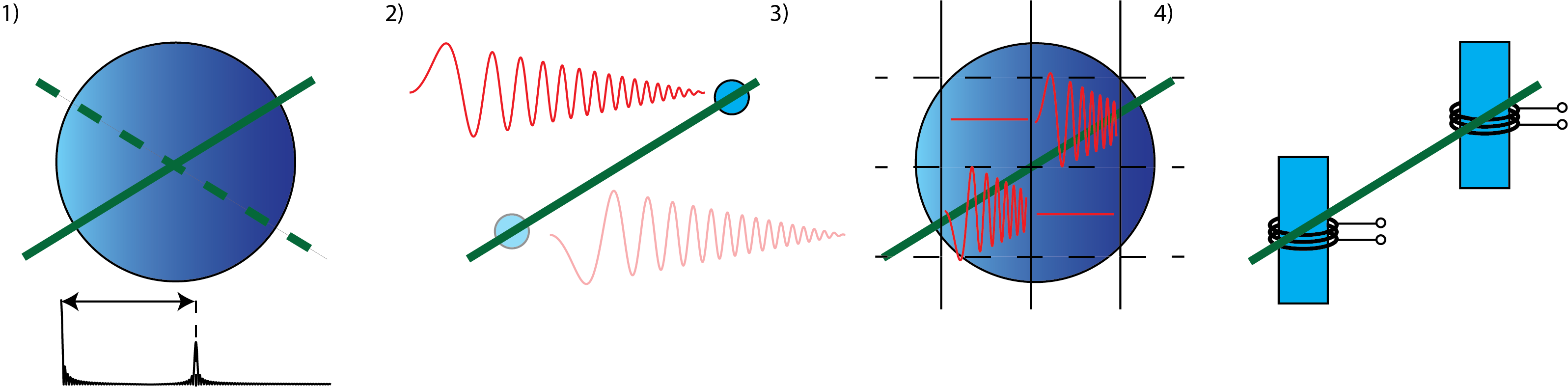
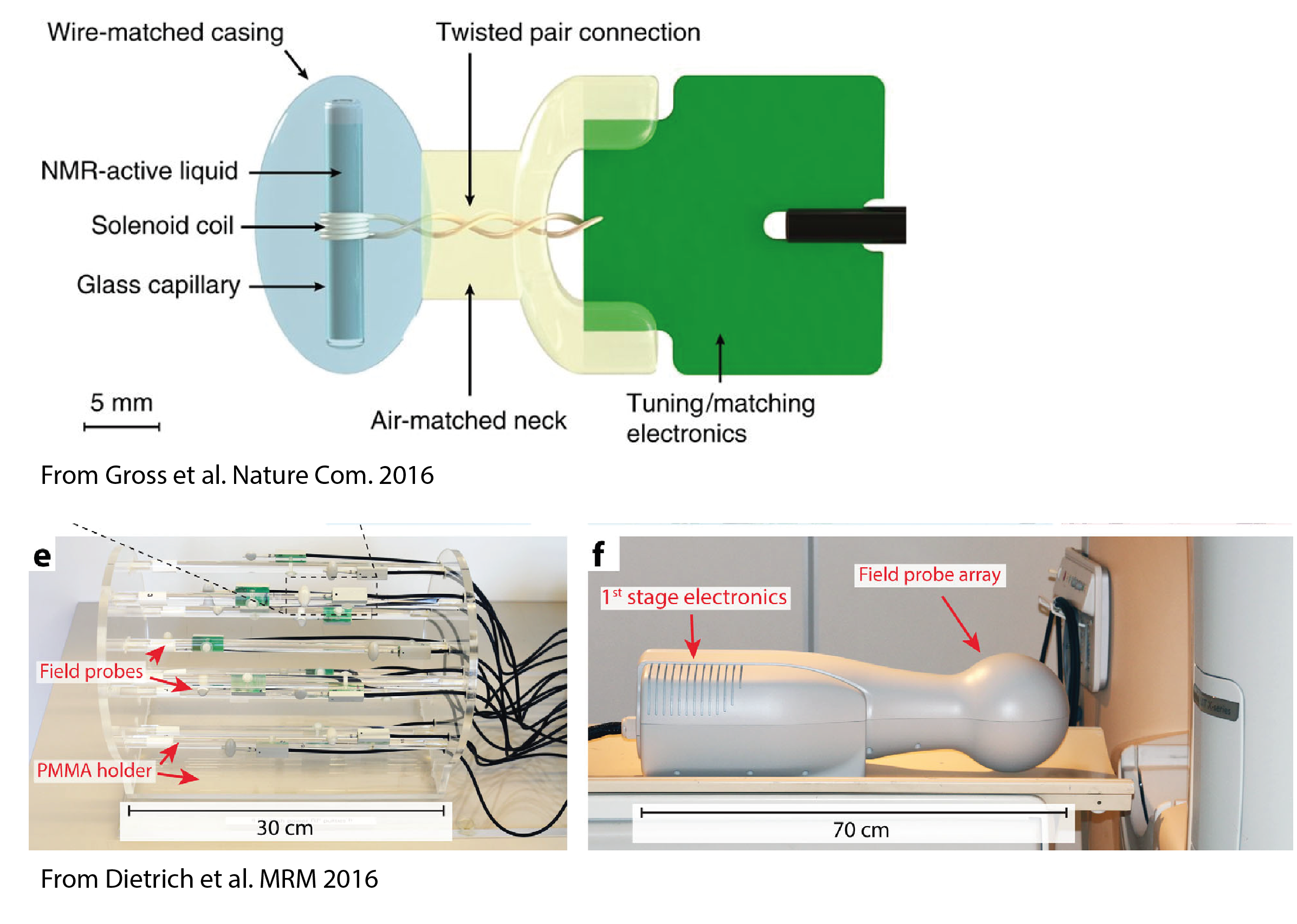
NMR based methods offer typically the highest accuracy for field measurements for MRI calibration purposes. They are all based on the effect that the phase of the first order MR coherences (EPR or NMR) accrues proportionally to the time integral of the induction field the spin is exposed to: $$\varphi(t)=\gamma \int |B(t)|dt$$ The simplest approach is to consider the phase evolution of an NMR active test sample, which is typically done for considering and stabilizing main magnet drift e.g. in high resolution NMR spectrometers in form of a spin lock. However, determining the behaviour of a gradient system requires a certain spatial resolution of the induced field. This can either be achieved (Fig.2) by considering the timing of echo formations under test gradients, scanning the sample or by employing slice selection or phase encoding [2-5]. Spatial selectivity can also be achieved by surrounding small, NMR active samples with separate receivers, so called field probes. The close coupling to the receiver provides also a very high SNR efficiency per unit sample volume, which is crucial to resolve test waveforms with high amplitudes and to operate under potential B0 non-uniformities with minimal dephasing.Field probe arrays
Due to their high isolation, field probes can be operated in parallel in an array configuration. Thereby each field probe sampling the field evolution resolves the space. Knowing the field at a set of positions ($$$B_p(t)$$$) the field inside the probe array [12] can be interpolated using an appropriate set of spatial basis functions ($$$B_i(r)$$$) each with a time course $$$J_i(t)$$$: $$B(r,t)=\sum_i B_i(r) \cdot J_i(t).$$ In a first step, the measurement of each probe at position $$$r_p$$$ have to be projected to the spatial basis: $$(B)_p=B_p(r_p, t)=\sum_i B_i(r_p) \cdot J_i (t)= (PJ)_p$$ $$(P)_{p i}=B_i(r_p), (J)_i = J_i(t)$$ $$J=P^+ B$$ It has to be noted, that the choice of basis function determines the representation of the dynamics. Choosing a set of basis functions along the degrees of freedoms of the system can therefore greatly simplify the representation of the dynamics. Employing gradient coordinates by calibrating the position of the probes with the static field offset induced by each gradient axis helps to separate static, spatial gradient non-linearity from dynamically induced field distortions.B0 field stability characterization
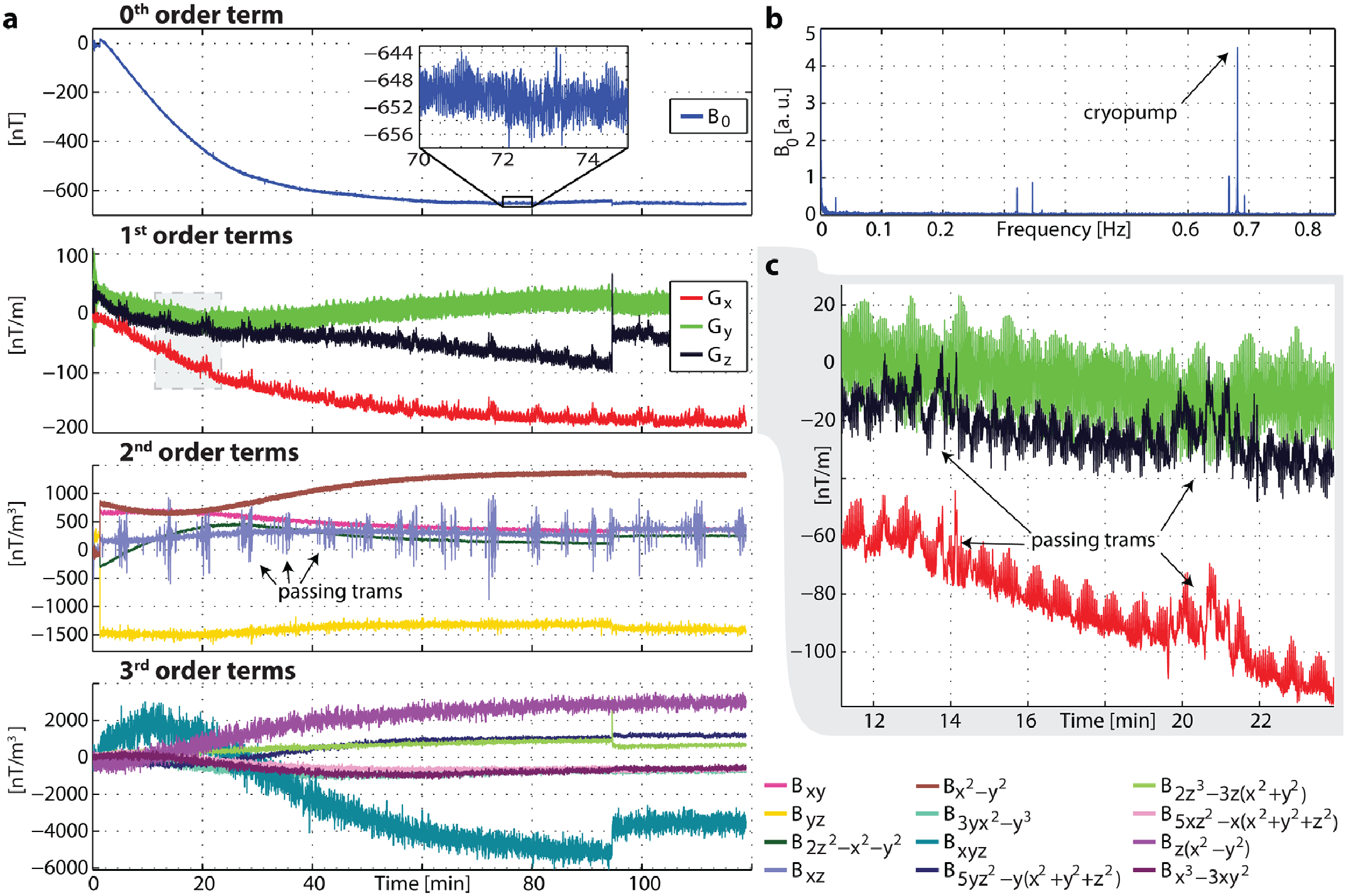
Typically employed super-conducting magnets offer a very high degree of uniformity and field stability. However, other components in the bore and on the magnet, such as gradient coils, shim irons etc. can induce signifficant field drifts as a function of their temperature (Fig.4).Gradient system characterization – A linear, time-invariant system approach
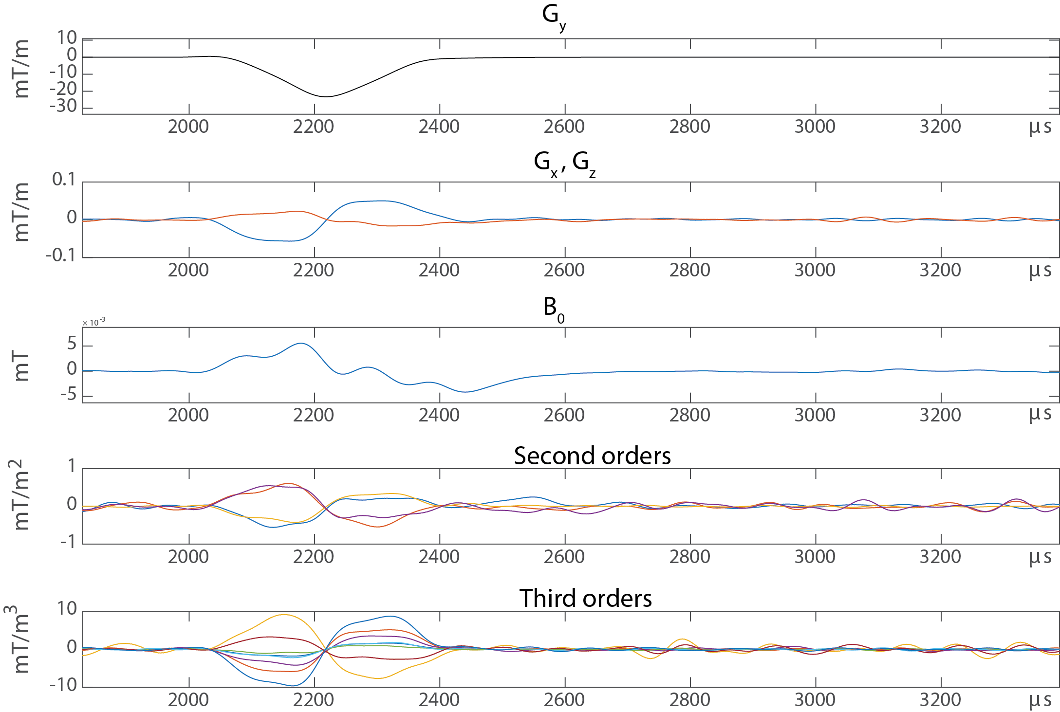
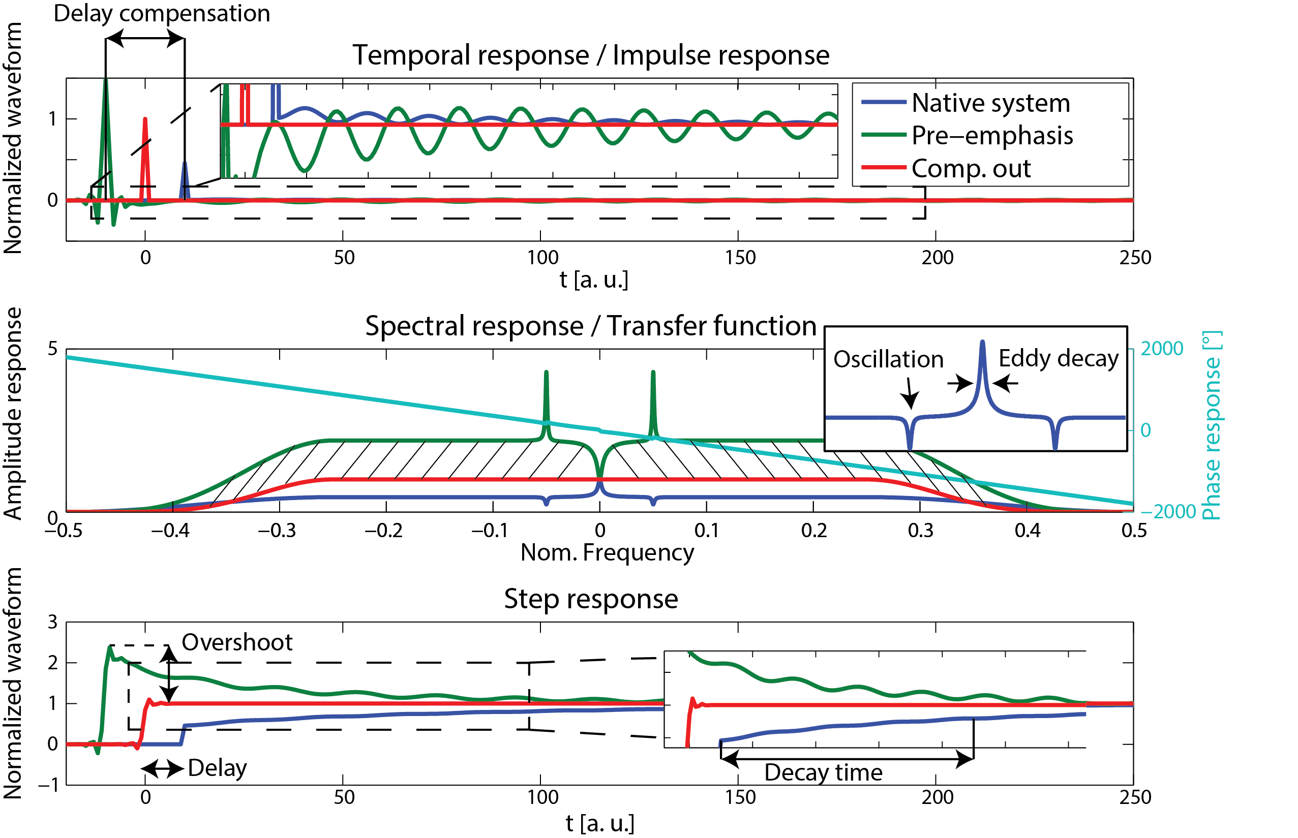
The goal of a system characterization is to predict the output of the system dependent on its given inputs. This knowledge can then be used for calibration, feedback adjustments, post-correction and sequence optimization. Fields induced by sources not under control of the scanner or that are not dependent on accessible variables cannot be considered for a calibration and represent therefore a constant source of potential confounders of the calibrated system’s output but also for the calibration procedure itself. However, for calibration purposes the MRI system has to be considered as time invariant and it remains to other means that other confounders are minimal. Additionally, the gradient and shim systems can be to a very large degree considered as linear systems, i.e. the field output is considered linearly dependent on the demand sent to the system [13]. Ensuring this linearity however is a critical effort in the hardware design and is ensured by very involved feedback driving circuits as mentioned above. As a consequence of the linearity and time invariance, the field output ($$$B(r,t) = \mathcal{F}^{-1}(b(r,\omega))$$$) is given as convolution of the demanded waveform ($$$ D(t) = \mathcal{F}^{-1}(d(\omega))$$$) and the impulse response function ($$$IR(r,t) = \mathcal{F}^{-1}(H(r,\omega))$$$) of the system: $$B(r,t) = D(t) \otimes IR(r,t),$$ or analogously in frequency domain: $$b(r,\omega) = d(\omega) \cdot H(r,\omega).$$ The calibration sequences characterizing the system have therefore to provide the data basis to determine the transfer function within the required bandwidth. This is achieved by recording the field output for a set of known inputs, which cover the required frequency span. The transfer function is then found by a deconvolution of the output with the input signal: $$H(r,\omega) = \frac {b(r,\omega)}{d(\omega)}.$$ In principle various test functions can be employed as input such as blips or frequency sweeps as long as the system is not driven to substantial non-linearity arising from amplitude or slew-rate limitations. Fig.5 shows an example for the response of a y gradient coil to a trapezoidal blip. The impulse response and equally the transfer functions contains a lot of information on delay, eddy currents oscillations etc. as depicted in Fig.6. The input waveform and the impulse responses can be decomposed into a basis set which yields: $$B(r,t) = \sum_{i=0…n} B_i(r) \cdot J_i(t) = \sum_{i=0…n, p=0…n} B_i(r) D_p(t) \otimes IR_{i,p}(t)$$, $$b(r,t)= \sum_{i=0…n, p=0…n} B_i(r) d_p(\omega) \cdot H_{i,p}(\omega).$$ The system’s response is then characterized by a matrix of transfer/response functions. The response of the channel to itself is characterized in the $$$ IR_{Iii}(t)$$$ functions, the cross-term couplings are represented in the off-diagonal functions. Note that the transfer functions of gradients and shim systems are sometimes misleadingly referred to as Gradient Impulse Response Functions.Feedforward compensation
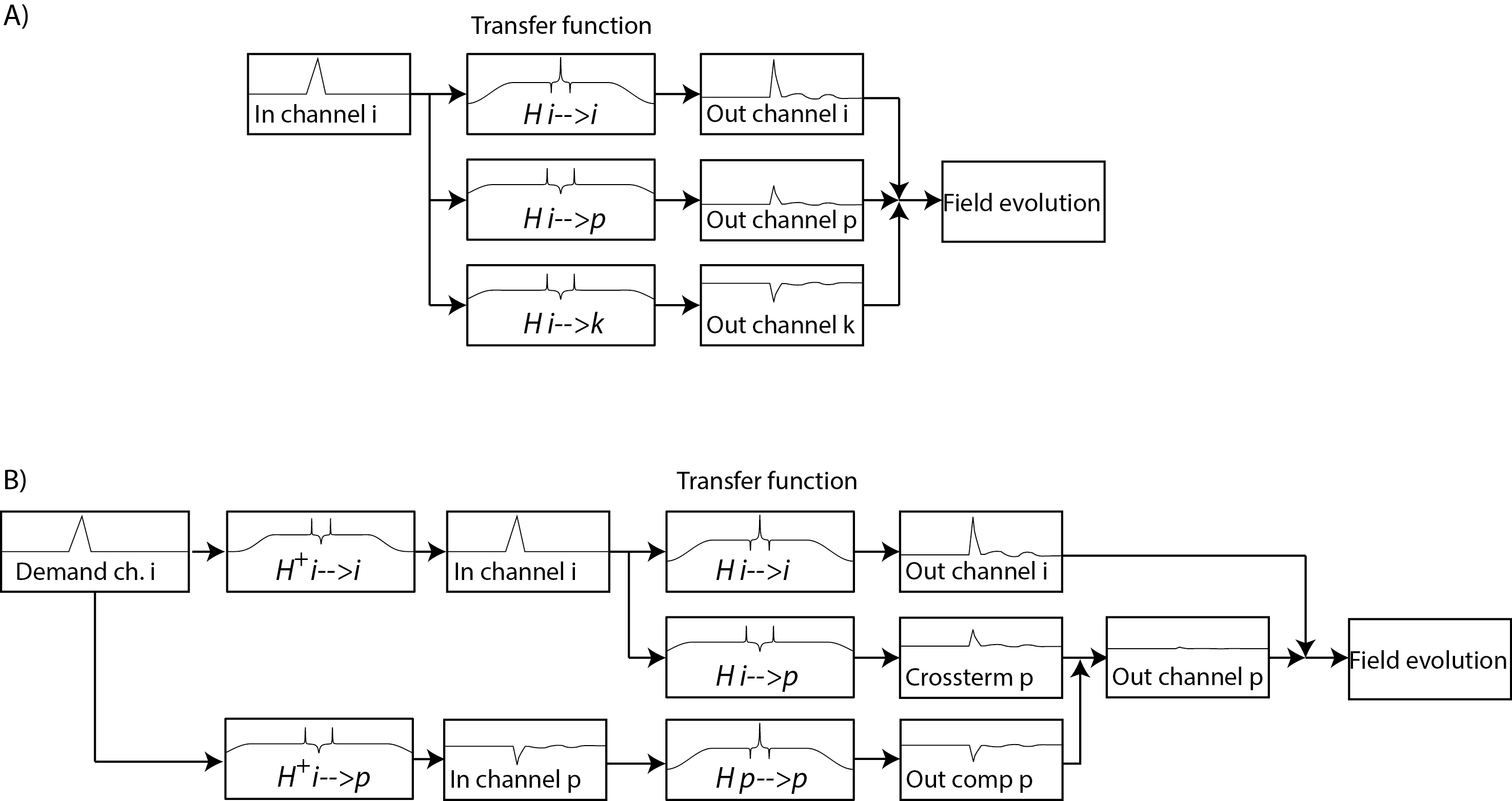
The basic idea of feedforward compensations is to pre-distort the requested waveform such that the field evolution at the output of the system will fit the request within the targeted bandwidth. For instance a delay can be compensated by playing out the waveform earlier such that it will arrive in time. Generally, each frequency component can be scaled and phased at the input based on its characterized response such that it will be equalized at the output. Such approaches are called pre-emphasis. Since eddy currents and other band-limiting effects lower the efficiency of the gradient system at higher frequencies, these components have to be scaled up in the demand sent to the amplifier, which results in a required overdrive in the pre-distorted waveform. The amplifier has consequently to produce higher output voltages or currents in order to speed up the ramping of the fields and to suppress cross terms. This in turn limits slewing and peak values for the not pre-emphasized waveform. Therefore it is important to limit the targeted response of each channel to the minimum required bandwidth by using a windowing function ($$$W(\omega)$$$) attenuating the request for high frequency components. Then the pre-distorted waveform ($$$D^C(t) = \mathcal{F}^{-1}(d^C(\omega)$$$) can be calculated by a deconvolution operation as also depicted in Fig.6: $$d^C(\omega) = \frac {d(\omega) \cdot W(\omega)}{H(\omega)} = d(\omega) \cdot H^+(\omega),$$ $$D^C(t) = D(t) \otimes IR^+(t),$$ where $$$H^+(\omega)=\frac{W(\omega)}{H(\omega)}$$$, and $$$IR^+(t) = \mathcal{F}^{-1} (H^+)$$$. Analogously cross-terms can be suppressed by inverting the transfer function matrix for each frequency (see Fig.7): $$H^+(\omega) _{i,p} = W(\omega) \left ( H(\omega)^ {-1} \right )_{i,p} \forall \omega.$$ Also here other channels have to allocate overhead power in order to compensate for the coupling. Therefore the inversion of the transfer matrix has to be carefully regularized by use of an appropriate pseudo-inverse ensuring a well-conditioned inverse at every frequency.Capturing deviations from time-invariant linear models
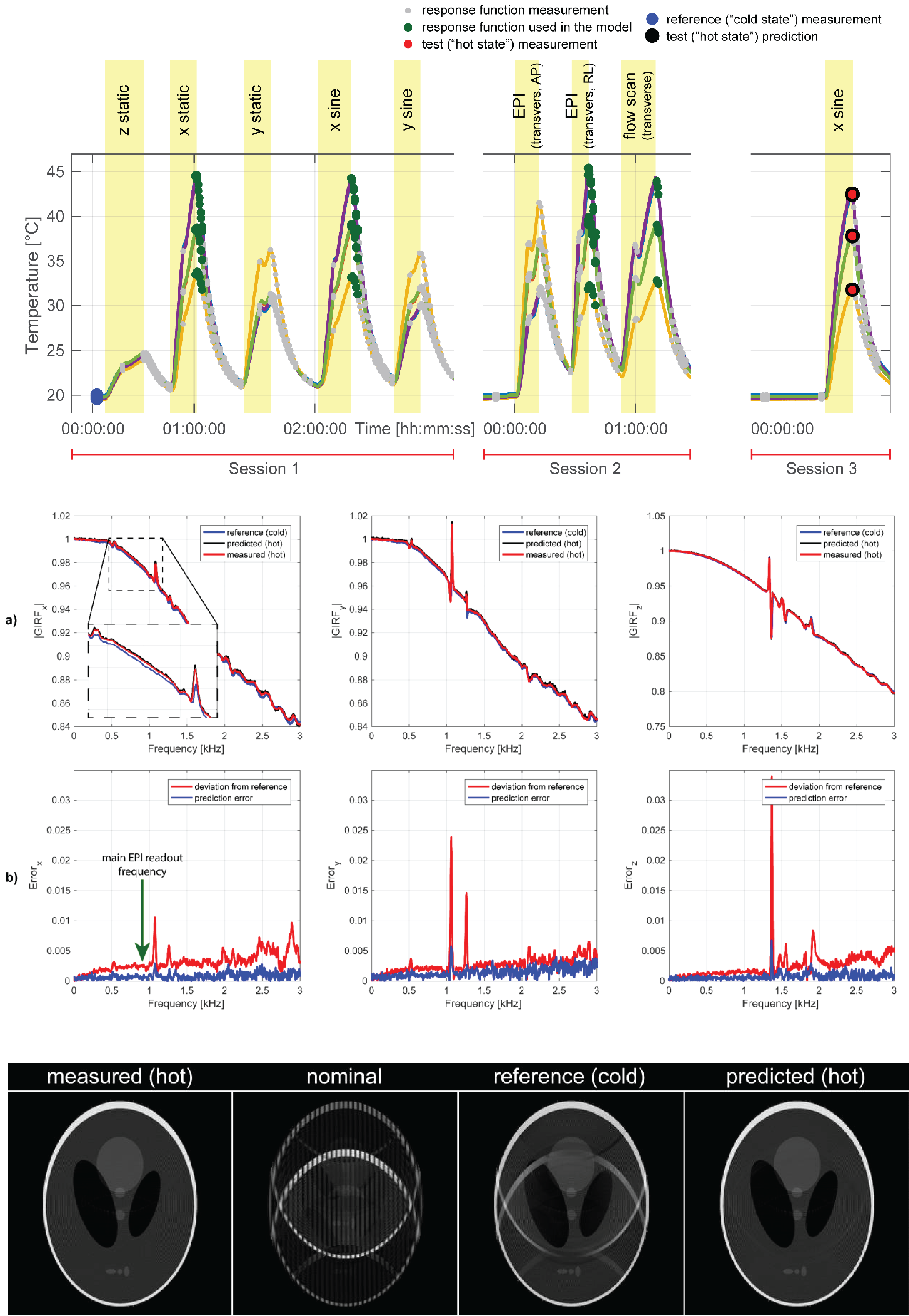
There are measurable and in some cases significant deviations from a linear and a time-invariant model. Non-linearities are mostly induced by the gradient amplifier. An effect of this sort is the leakage of a ripple from the switch mode output stages. These ripples are typically found at frequencies between 20 kHz and 200 kHz irrespective of the input signal violating the linearity requirement. However, due to their high frequency the influence on the image encoding is subliminal. Compression is an effect that has more practical relevance. Compression means that the amplifier does not output a multiple of the input waveform. Typically, waveform sections involving high slew rates or amplitudes have a slightly lower gain. Consequently, the output current curve is slightly compressed. In current MRI systems these compressions lie in the order of several per mill of the current [14]. However, the appearance of the consequent modulation terms can hamper the acquisition of the linear response during the calibration process. Time-invariance is, given no changes are made to the system, mostly broken by temperature induced alterations. Magnitude and lifetime of eddy currents are dependent on the conductivity of the material, which in turn depends on its temperature. Another main contribution to temperature induced system alterations results from changing mechanical properties. In particular, the gradient tube’s fibre-reinforced resins soften significantly over the temperature range of operation by which mechanical resonances of the tube shift and broaden. Fig.8 collected from [15] shows the effect of deliberately induced temperature variations on the linear response and EPI imaging. A key advantage of field probe based techniques is that the measurements, even including higher spatial orders, is single shot and does not require any signal generation or localization from the scanner itself. By this, the measurement of the system properties minimally interfere with scanner itself, e.g. by adding additional heating or allowing a system cool-down during measurement. In turn drifts of the system behaviour and background field can be resolved and thereby isolated from the system characterization.Acknowledgements
No acknowledgement found.References
1. Schmitt, F., Correction of Geometrical Distortions in MR-images, in Computer Assisted Radiology / Computergestützte Radiologie, H. Lemke, et al., Editors. 1985, Springer Berlin Heidelberg. p. 15-23.
2. Davies, N.P. and P. Jezzard, Calibration of gradient propagation delays for accurate two-dimensional radiofrequency pulses. Magnetic Resonance in Medicine, 2005. 53(1): p. 231-236.
3. Jezzard, P., A.S. Barnett, and C. Pierpaoli, Characterization of and correction for eddy current artifacts in echo planar diffusion imaging. Magnetic Resonance in Medicine, 1998. 39(5): p. 801-812.
4. Mason, G.F., et al., A Method to measure arbitrary k-space trajectories for rapid MR imaging. Magnetic Resonance in Medicine, 1997. 38(3): p. 492-496.
5. Schmithorst, V.J. and B.J. Dardzinski, Automatic gradient preemphasis adjustment: A 15‐minute journey to improved diffusion‐weighted echo‐planar imaging. Magnetic Resonance in Medicine, 2002. 47(1): p. 208-212.
6. Duyn, J.H., et al., Simple Correction Method for k-Space Trajectory Deviations in MRI. Journal of Magnetic Resonance, 1998. 132(1): p. 150-153.
7. Alley, M.T., G.H. Glover, and N.J. Pelc, Gradient characterization using a Fourier-transform technique. 1998. 39(4): p. 581-587.
8. De Zanche, N., et al., NMR probes for measuring magnetic fields and field dynamics in MR systems. Magnetic Resonance in Medicine, 2008. 60(1): p. 176-186.
9. Barmet, C., et al., A transmit/receive system for magnetic field monitoring of in vivo MRI. Magnetic Resonance in Medicine, 2009. 62(1): p. 269-276.
10. Dietrich, B., et al., A field camera for MR sequence monitoring and system analysis. Magn Reson Med, 2015.
11. Gross, S., et al., Dynamic nuclear magnetic resonance field sensing with part-per-trillion resolution. Nature Communications, 2016. 7: p. 13702.
12. Barmet, C., N.D. Zanche, and K.P. Pruessmann, Spatiotemporal magnetic field monitoring for MR. Magnetic Resonance in Medicine, 2008. 60(1): p. 187-197.
13. Vannesjo, S.J., et al., Gradient system characterization by impulse response measurements with a dynamic field camera. Magnetic Resonance in Medicine, 2012. 69(2): p. 583-593.
14. Nussbaum, J., et al. Nonlinearity and thermal effects in gradient chains: a cascade analysis based on current and field sensing. in Proc Intl Soc Magn Reson Med. 2019. Montreal, Canada.
15. Dietrich, B.E., et al. Thermal Variation and Temperature-Based Prediction of Gradient Response. in Proc Intl Soc Magn Reson Med. 2017. Honolulu, USA. 16. Duerst, Y., et al., Real-time feedback for spatiotemporal field stabilization in MR systems. Magnetic Resonance in Medicine, 2014. 73(2): p. 884–893.
17. Buonocore, M.H. and L. Gao, Ghost artifact reduction for echo planar imaging using image phase correction. Magnetic Resonance in Medicine, 1997. 38(1): p. 89-100.
18. Vannesjo, S.J., et al., Image reconstruction using a gradient impulse response model for trajectory prediction. Magnetic Resonance in Medicine, 2015: p. n/a-n/a.
19. Wilm, B.J., et al. High-Resolution Single-Shot Spiral Imaging using Magnetic Field Monitoring and its Application to Diffusion Weighted MRI. in Proc Intl Soc Magn Reson Med. 2015. Toronto, Canada.
20. Wilm, B.J., et al., Higher order reconstruction for MRI in the presence of spatiotemporal field perturbations. Magnetic Resonance in Medicine, 2011. 65(6): p. 1690-1701.
Figures