Synopsis

While the spin is an intrinsic quantum mechanical property of elementary particles, quantum mechanics are not necessarily required to describe many of the basic processes of NMR or MRI. This lecture aims at providing an intuitive understanding of the NMR phenomenon (including spin precession, RF excitation and relaxation) in conjunction with a brief overview of the basic components of MR systems.

Target Audience

Objectives

Following this lecture, audience members should be able to describe:

• the concepts of spin precession and net magnetization
• the basic components of an MRI system
• the mechanisms of RF excitation and signal reception
• the concept of relaxation and the evolution of the magnetization using Bloch equations
  

Precession, Longitudinal Relaxation and Net Magnetization

While the spin is an intrinsic quantum mechanical property of elementary particles, quantum mechanics are not necessarily required to describe many of the basic processes of NMR or MRI.

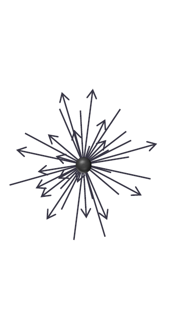
To start with this classical description, let’s think about the spin as an intrinsic angular momentum leading to a circulating electric current (1). The angular momentum is hence associated with a magnetic moment $$$\vec{\mu}$$$. Spins in an ensemble (e.g. a sample) are in a thermal equilibrium, and we can assume them to be arbitrarily oriented so that all nuclear magnetic moments cancel out (Fig. 1).

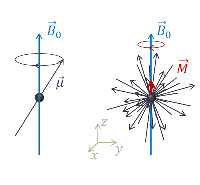
Once the spins get placed in an external magnetic field $$$\vec{B_{0}}$$$, the spins behave like spinning tops in a gravitational field and start to precess around the axis of the magnetic field at the Larmor frequency

$$\omega_{0} = \gamma B_{0}$$

with γ being the gyromagnetic ratio, a specific constant for each nucleus.

Over time, a new thermal equilibrium with a typically small non-zero net magnetization M₀ will form (Fig. 2). We can think of thermal energy (energy exchange between the nuclei) slowly altering the previously mentioned isotropic orientation of the magnetic moments slightly pushing the spins towards a precession angle with lower magnetic energy (2). We call this process longitudinal or T₁ relaxation and it can be used to create contrast in MRI. Assuming the static magnetic field is aligned along the z-axis, we can write:

$$\frac{dM_{z}}{dt}=\frac{1}{T1}(M_{0}-M_{z})$$

where T₁ defines the tissue specific longitudinal relaxation time constant. The static magnetic field B₀ determines the overall sample polarization and hence the achievable signal-to-noise ratio (SNR).

Clinical high-field MRI systems (B₀ > 1T) typically use superconducting niobium titanium coils, cooled by liquid Helium in a cryostat to generate the high static magnetic field. Lower magnetic fields can also be generated by electromagnets or by permanent magnets. The systems are usually shielded to remove the outside stray-field. Shimming by means of additional superconducting coils, resistive coils or passive shim material is employed to improve the spatial uniformity of the field.

RF Excitation and Signal Reception

The net magnetization can be manipulated by applying an additional spatially uniform radio frequency (RF) field $$$\vec{B_{1}(t)}$$$, perpendicular to $$$\vec{B_{0}}$$$, tuned to the Larmor frequency ω₀. The spins will now precess about the effective magnetic field $$$\vec{B} = \vec{B_{0}} + \vec{B_{1}(t)}$$$ following the equation:

$$\frac{dM}{dt}=\gamma \vec{M}\times \vec{B}$$

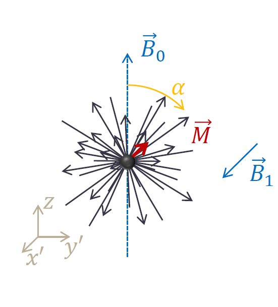
It is common to look at this NMR experiment from the so-called rotating frame of reference, a reference frame rotating at the Larmor frequency about the z-axis. Here, $$$\vec{B_{1}}$$$ is stationary and also the only effective field so the spins and magnetization will precess about it. Starting from the equilibrium state, $$$\vec{M_{0}}$$$ will simply rotate about the axis of B₁ (Fig. 3). The angle of rotation α is known as flip angle and is determined by the power and duration of the B₁ field.

After applying such an RF pulse, the magnetization vector will have a component perpendicular to the static magnetic field. This transverse magnetization M_xy can be detected as an oscillating signal in a receiver coil.

In most clinical MR systems, the B₁ RF fields are generated by a (birdcage) volume coil inside the magnet bore driven by RF power amplifiers. In general, the coil can also be used for signal reception; however, the use of local receiver arrays with multiple smaller elements is beneficial in terms of SNR and facilitates parallel imaging. The received signals get amplified and digitized before image reconstruction or post-processing. At ultra-high field (B₀ ≥ 7T), body coils are unsuitable and RF transmission is performed using local transceiver arrays, which can also be used for parallel transmission. RF power deposition into tissue can be characterized by the so called specific absorption rate (SAR). Constant SAR monitoring is required to keep the power deposition within regulatory limits.

Transverse Relaxation, Spin Dephasing and Bloch Equations

The transverse magnetization is subject to a separate relaxation process, which is called transverse or T₂ relaxation. The spins introduce dynamic fluctuations in the local magnetic field of their neighbours, which causes a variation in the local precessional frequencies and hence dephasing of the spins. The transverse magnetization decays with the tissue-specific time constant T₂. In the rotating frame of reference, the decay simplifies to:

$$\frac{dM_{xy}}{dt} = -\frac{1}{T_{2}}M_{xy}$$

Additional static local magnetic field inhomogeneities accelerate this spin dephasing, shortening the T₂ relaxation process. The shortened relaxation is described by the time constant T₂*.

The previously mentioned equations are essentially parts of the full set of Bloch equations (3), which can be used to fully describe the behaviour of the magnetization and are outlined below:

$$\frac{dM_{x}}{dt} = \gamma(M_{y}B_{z}-M_{z}B_{y})-\frac{1}{T_{2}}M_{x}$$

$$\frac{dM_{y}}{dt} = \gamma(M_{z}B_{x}-M_{x}B_{z})-\frac{1}{T_{2}}M_{y}$$

$$\frac{dM_{z}}{dt} = \gamma(M_{x}B_{y}-M_{y}B_{x})-\frac{M_{0}-M_{z}}{T_{1}}$$

Spin dephasing and rephasing is also an integral mechanism in the process of echo generation and spatial encoding (covered by a separate lecture) in MRI. The latter is realized by applying small magnetic gradient fields on the order of a few mT/m in addition to the static magnetic field B₀. The gradient fields are designed to vary the main magnetic field B₀ linearly along three orthogonal spatial directions x, y, and z. Hence, their field vector is aligned with the main magnetic field. Gradient switching is associated with acoustic noise and peripheral nerve stimulation. The latter is a limiting factor in a large number of applications. Gradient pre-emphasis can be employed to counterbalance distorting eddy-current effects.

Acknowledgements

References

[1] Haacke EM, Brown RW, Thompson MR, Venkatesan R, Magnetic Resonance Imaging: Physical Principles and Sequence Design, Wiley-Liss (1999)

[2] Hanson, Concepts in Magnetic Resonance Part A, 32A:329-340 (2008)

[3] Bloch, Nuclear Induction, Phys. Rev. 70, 460 (1946)