From Magnetism to Fieldmaps & Back
1University College London, United Kingdom
Synopsis
Tissue magnetic susceptibility can be calculated from gradient-echo phase images using quantitative susceptibility mapping (QSM). I will explain the relationship between phase and susceptibility and how we can use this to map tissue susceptibility. Several clinical applications of QSM are emerging based on its sensitivity to tissue iron, myelin and deoxyhaemoglobin content.
What Is Susceptibility?
Susceptibility is an intrinsic bulk material or tissue property that determines how a material or tissue will interact with and behave in an applied magnetic field [1]. Tissues with positive susceptibility values are paramagnetic (i.e. their magnetisation increases with the applied magnetic field strength) and those with negative susceptibility values are diamagnetic. We are interested in tissue magnetic susceptibility because it is directly related to the tissue composition and microstructure. This means susceptibility maps have the potential to yield interesting information on pathophysiology-related changes in tissue composition and microstructure.
How To Measure Tissue Magnetic Susceptibility?
The key to measuring susceptibility(c) is that the phase of the complex MRI signal in simple T2*-weighted gradient-echo MRI sequences is directly determined by the underlying tissue magnetic susceptibility [2, 3]. It is useful to picture a small spherical point ‘source’ with a different susceptibility to its surroundings, in a magnetic field (B0 along the z direction). The source will produce small magnetic field perturbations that have a dipolar distribution (d(r)) (figure 1). A more complicated susceptibility distribution c(r) will lead to a more complicated field distribution DBz(r) which can be understood as the sum or superposition of many dipole fields from many small point sources of susceptibility. This can be expressed mathematically as follows:
DBz(r) = B0 . d(r) Ä c(r) (1)
which means that, if we knew the susceptibility distribution inside tissue (c(r)) it would be possible to calculate the field distribution DBz(r) by convolving c(r) with the unit dipole field kernel d(r).
We are able to measure the field perturbations induced by tissue magnetic susceptibility distributions because they are linearly related to the phase of the complex MRI signal in T2*-weighted gradient-echo MRI sequences. The phase f(r) is related to DBz(r) according to
f(r,TE) = gDBz(r).TE + f0(r) (2)
where g is the gyromagnetic ratio, TE is the echo time and f0(r) is the phase at TE=0 (figure 2).
This means that the rich contrast available in these phase images [4], which were often discarded in the past, can be used to calculate (based on equations 1 and 2) maps of the underlying tissue magnetic susceptibility distribution.
The problem with using phase images as they are is that the phase contrast is non-local, extending beyond the structures of interest, and also depends on the orientation of these structures with respect to the main magnetic field B0. QSM overcomes these disadvantages [5].
Conceptual Stages in QSM
This process of susceptibility mapping (often labelled Quantitative Susceptibility Mapping (QSM) (figure 3) ) has developed rapidly over the last few years and has been described in several recent review papers [6-9]. Complexities in QSM include: Phase images suffer from phase wrapping (as the phase is an angle defined only between ± p, figure 2) and there are a large variety of unwrapping algorithms available, e.g. [10-12], each with advantages and drawbacks. The measured phase also depends upon imaging parameters such as the echo time (TE, Equation 2) and the voxel aspect ratio [13, 14]. The phase will also be affected by hardware differences in vendor systems such that there are two phase sign conventions [15]. Furthermore, when using multiple channel radio frequency coils, it is crucial that the phase images from each of the coil channels is combined correctly to reconstruct an accurate phase image [11, 16] otherwise intractable artifacts known as open-ended fringe lines or phase singularities can occur. It is also important to obtain the most accurate estimate of DBz(r) by fitting over phase images f(r,TE) measured at multiple echo times [17-19].
The next step in calculating susceptibility maps is to remove large-scale background phase variations caused primarily by the relatively large susceptibility difference between tissue and air in cavities and outside the body. These background phase variations are often much larger than the susceptibility-induced phase differences of interest between different tissues and there are now a wide variety of techniques for removing them, e.g. [20-22]. Masking out noisy phase in areas where there is no MRI signal (e.g. outside the body) is often a prerequisite for applying (unwrapping and) background field removal. Note that, primarily as a result of removing background phase variations, the contrast observed in susceptibility maps is relative rather than absolute.
The final step in calculating susceptibility images from these processed phase images is to solve the inverse problem i.e. calculate the susceptibility distribution c(r) from the measured phase images f(r). A large variety of methods have been developed to overcome the ill-posed or ill-conditioned nature of the inverse problem or regularize it. K-space based algorithms do this by removing, substituting or correcting the data inside ill-conditioned regions in k-space. Some earlier methods required acquisitions at multiple angles [23] with the majority of newer methods needing acquisition at just a single orientation [24, 25] with respect to the main magnetic field (B0). These single-orientation methods are preferable due to the additional time and discomfort (or impossibility of positioning for human applications in the body) involved in acquiring images with the region of interest at several orientations with respect to B0. Although we have described several separate conceptual steps in QSM, practically or computationally, these can sometimes be combined into fewer steps [26, 27] or even a single step [28].
Conclusions
There are a large variety of QSM algorithms available, each with relative merits and disadvantages. The resulting susceptibility maps have important advantages over the phase images from which they were calculated; they overcome the non-local and orientation-dependent nature of the contrast in phase images [5], allowing improvements in the visualisation of tissue structure and composition. These advantages also stand against the earlier and more widespread precursor to QSM known as susceptibility weighted imaging (SWI) in which phase images are unwrapped, filtered and multiplied with the corresponding magnitude images to emphasise susceptibility-induced phase changes [29]. A common practical pitfall is the acquisition of images with insufficient resolution and/or coverage [30] for QSM. It is important to ensure that the field perturbations DBz(r) induced by susceptibility sources c(r) are sufficiently sampled so that they can be accurately inverted.
Acknowledgements
No acknowledgement found.References
1. J.F. Schenck, The role of magnetic susceptibility in magnetic resonance imaging: MRI magnetic compatibility of the first and second kinds. Medical Physics, 1996. 23(6): 815-850.
2. R. Salomir, et al., A fast calculation method for magnetic field inhomogeneity due to an arbitrary distribution of bulk susceptibility. Concepts in Magnetic Resonance Part B-Magnetic Resonance Engineering, 2003. 19B(1): 26-34.
3. J.P. Marques and R. Bowtell, Application of a Fourier-based method for rapid calculation of field inhomogeneity due to spatial variation of magnetic susceptibility. Concepts in Magnetic Resonance Part B: Magnetic Resonance Engineering, 2005. 25B(1): 65-78.
4. J.H. Duyn, et al., High-field MRI of brain cortical substructure based on signal phase. Proc Natl Acad Sci U S A, 2007. 104(28): 11796-801.
5. K. Shmueli, et al. The Dependence of Tissue Phase Contrast on Orientation Can Be Overcome by Quantitative Susceptibility Mapping. in Proc ISMRM, 2009. Honolulu, Hawai'i, USA, 17, p. 466.
6. E.M. Haacke, et al., Quantitative susceptibility mapping: current status and future directions. Magn Reson Imaging, 2015. 33(1): 1-25.
7. C. Liu, et al., Susceptibility-weighted imaging and quantitative susceptibility mapping in the brain. J Magn Reson Imaging, 2015. 42(1): 23-41.
8. Y. Wang and T. Liu, Quantitative susceptibility mapping (QSM): Decoding MRI data for a tissue magnetic biomarker. Magn Reson Med, 2015. 73(1): 82-101.
9. A. Deistung, et al., Overview of quantitative susceptibility mapping. NMR Biomed, 2017. 30(4): e3569.
10. M. Jenkinson, Fast, automated, N-dimensional phase-unwrapping algorithm. Magnetic Resonance in Medicine, 2003. 49(1): 193.
11. S.D. Robinson, et al., An illustrated comparison of processing methods for MR phase imaging and QSM: combining array coil signals and phase unwrapping. NMR in Biomedicine, 2016.In Press.
12. A. Karsa and K. Shmueli, SEGUE: a Speedy rEgion-Growing algorithm for Unwrapping Estimated phase. IEEE Trans Med Imaging, 2019.In Press.
13. Y.B. Xu and E.M. Haacke, The role of voxel aspect ratio in determining apparent vascular phase behavior in susceptibility weighted imaging. Magnetic Resonance Imaging, 2006. 24(2): 155-160.
14. A. Deistung, et al., Susceptibility weighted imaging at ultra high magnetic field strengths: theoretical considerations and experimental results. Magn Reson Med, 2008. 60(5): 1155-68.
15. G.E. Hagberg, et al., The sign convention for phase values on different vendor systems: definition and implications for susceptibility-weighted imaging. Magnetic Resonance Imaging, 2010. 28(2): 297-300.
16. K. Eckstein, et al., Computationally Efficient Combination of Multi-channel Phase Data From Multi-echo Acquisitions (ASPIRE). Magnetic Resonance in Medicine, 2018. 79(6): 2996-3006.
17. T. Liu, et al., Nonlinear formulation of the magnetic field to source relationship for robust quantitative susceptibility mapping. Magn Reson Med, 2013. 69: 467-476.
18. E. Biondetti, et al. Application of Laplacian-based Methods to Multi-echo Phase Data for Accurate Susceptibility Mapping. in Proc ISMRM, 2016. Singapore, 24, p. 1547.
19. E. Biondetti, et al. Evaluating The Accuracy of Susceptibility Maps Calculated from Single-Echo versus Multi-Echo Gradient-Echo Acquisitions. in Proc ISMRM, 2017. Honolulu, Hawaii, USA, 25.
20. T. Liu, et al., A novel background field removal method for MRI using projection onto dipole fields (PDF). NMR in Biomedicine, 2011. 24(9): 1129-1136.
21. F. Schweser, et al., Quantitative imaging of intrinsic magnetic tissue properties using MRI signal phase: an approach to in vivo brain iron metabolism? Neuroimage, 2011. 54(4): 2789-807.
22. F. Schweser, et al., An illustrated comparison of processing methods for phase MRI and QSM: removal of background field contributions from sources outside the region of interest. NMR Biomed, 2017. 30(4).
23. T. Liu, et al., Calculation of susceptibility through multiple orientation sampling (COSMOS): a method for conditioning the inverse problem from measured magnetic field map to susceptibility source image in MRI. Magn Reson Med, 2009. 61(1): 196-204.
24. K. Shmueli, et al., Magnetic susceptibility mapping of brain tissue in vivo using MRI phase data. Magn Reson Med, 2009. 62(6): 1510-22.
25. S. Wharton, et al., Susceptibility mapping in the human brain using threshold-based k-space division. Magn Reson Med, 2010. 63(5): 1292-304.
26. F. Schweser, et al., Toward online reconstruction of quantitative susceptibility maps: superfast dipole inversion. Magn Reson Med, 2013. 69(6): 1582-94.
27. W. Li, et al., Integrated Laplacian-based phase unwrapping and background phase removal for quantitative susceptibility mapping. NMR Biomed, 2014. 27(2): 219-27.
28. I. Chatnuntawech, et al., Single-step quantitative susceptibility mapping with variational penalties. NMR in biomedicine, 2017. 30(4): 10.1002/nbm.3570.
29. E.M. Haacke, et al., Susceptibility weighted imaging (SWI). Magn Reson Med, 2004. 52(3): 612-8.
30. A. Karsa, et al., The effect of low resolution and coverage on the accuracy of susceptibility mapping. Magn Reson Med, 2019. 81(3): 1833-1848.
Figures
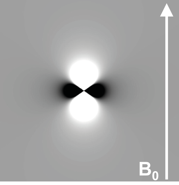
Figure 1: Magnetic Dipole Field (d(r))
Field perturbations DBz(r) associated with a point source with a susceptibility greater than that of the surrounding material placed in a magnetic field B0. Note that the dipole field is oriented along B0. This is the basis for the orientation dependence of the MRI phase.
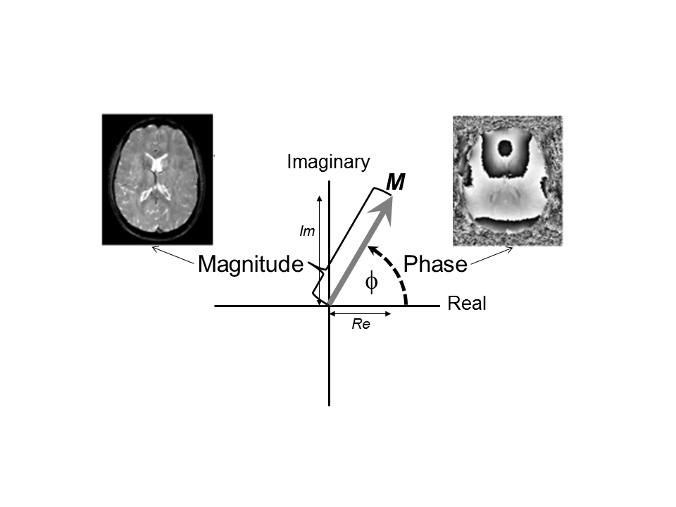
Figure 2: Phase in MRI
The magnetisation vector (M) precesses in the transverse (x-y) plane which can also be understood as the complex (real-imaginary) plane. The magnetisation (or MRI signal) is complex, having a magnitude and a phase. The length of the magnetisation vector is used in conventional T2*-weighted MRI to form the magnitude image. The angle that the magnetisation vector makes (dashed line) is the phase (f) and can be used to form a phase image. The magnetisation vector precesses in the transverse plane at an angular velocity ω = gDBz(r) which helps to explain equation 2.
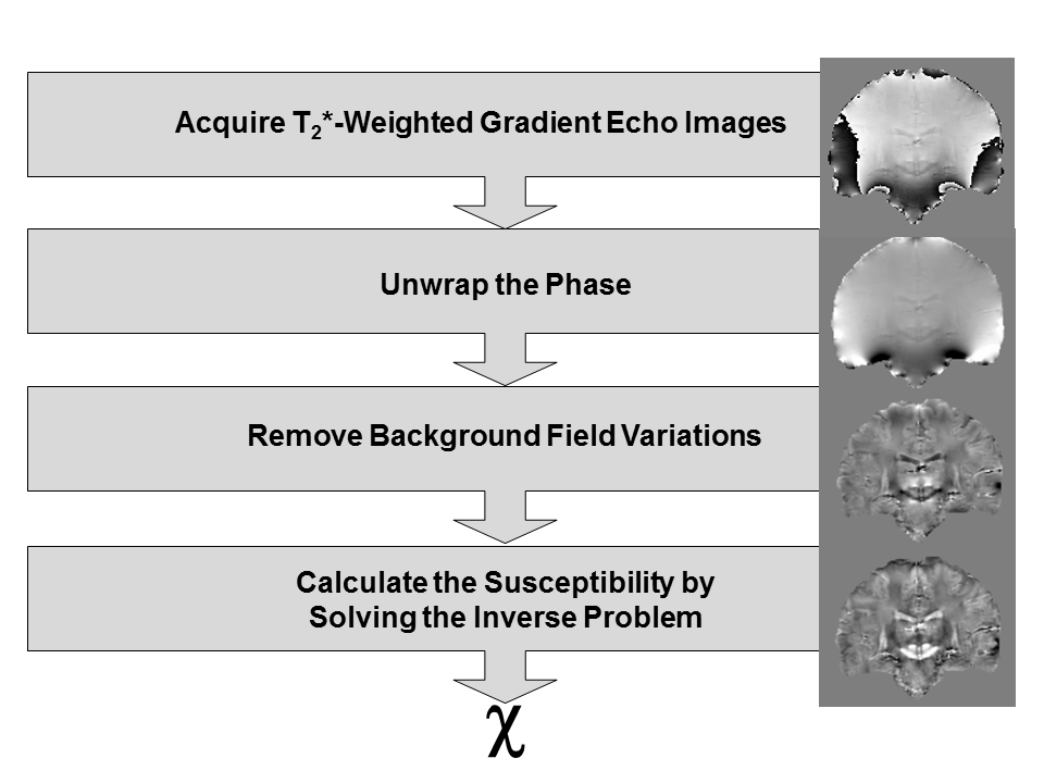
Figure 3: The Stages in Quantitative Susceptibility Mapping
All stages are illustrated with coronal brain images of a healthy human volunteer acquired at 3 Tesla. After acquisition, the phase is unwrapped (unwrapped image, 2nd row). Background field perturbations are removed to reveal the field perturbations induced by subtle tissue magnetic susceptibility differences (local field map, 3rd row). Finally, regularisation methods are applied to solve the inverse problem and provide a tissue magnetic susceptibility map (bottom row). This is relative rather than absolute because of the background field removal step.