5047
Discrete Laplacian Estimation Using Projection onto ROtating Median Sets (PROMS) for MR Electrical Property Tomography1Electronics and Information Engineering, Korea University, Seoul, Korea, Republic of, 2Korea Artificial Organ Center, Korea University, Seoul, Korea, Republic of, 3ICT Convergence Technology for Health and Safety, Korea University, Sejong, Korea, Republic of, 4Research Institute for Advanced Industrial Technology, Korea University, Sejong, Korea, Republic of, 5Korea Basic Science Institute, Cheongju, Chungbuk, Korea, Republic of, 6Corresponding author, ohch@korea.ac.kr, Korea, Republic of
Synopsis
The novel contrast mechanism,
Introduction
MR Electrical Property Tomography (MREPT) is the non-invasive imaging technique for estimating electrical properties of tissue using MRI. Although MREPT has a potential for diagnosis or treatment monitoring, the current extraction algorithm is limited in solving the governing equation completely and its high noise sensitivity causes the large errors in calculating Laplacian.1 To overcome the limitations, in recent studies many advanced reconstruction algorithms have been proposed for EPT.2-6 In this study, we propose a new Laplacian approximation using Projection onto ROtating Median Sets (PROMS) which reduces not only noise amplifications in Laplacian operation, but also prevents the boundary loss during iterative Median projections.Methods
1. Generalized Median Sets for Laplacian Estimation
The one-dimensional Laplacian kernel, L, can be represented as a difference of the Mean and identity kernels:
$$ L=\left[1 -2 1\right]=3\times(\frac{1}{3}\times\left[1 1 1\right]-\left[0 1 0\right]) $$
In this equation, for noisy images, the mean can be approximated from the Median value. Then the Laplacian can be estimated from the difference of two Median kernels with higher and lower center weights. It can be simply generalized as:
$$ \frac{1}{n_{L}}\times M_{L}-\frac{1}{n_{H}}\times M_{H}=\frac{W_{H}-W_{L}}{n_{H}n_{L}}L $$
where the center weighted Median kernel, $$$M_{H}$$$ and $$$M_{L}$$$ , whose components are $$$ [1 W_{H} 1]$$$ and $$$[1 W_{L} 1]$$$ with higher and lower weighting values, $$$W_{H}$$$ , and $$$W_{L}$$$, and normalizing constant, $$$n_{H}$$$ and $$$n_{L}$$$ is sum of all components in $$$M_{H}$$$ and $$$M_{L}$$$.
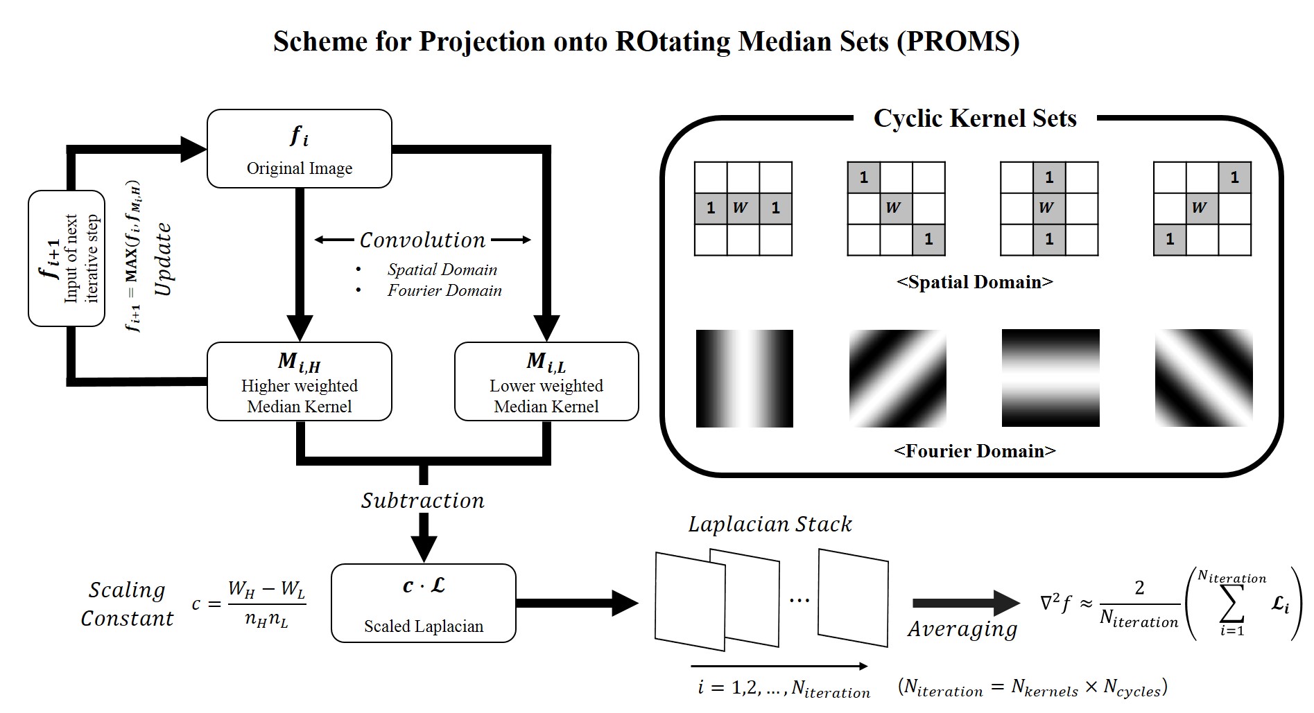
2. Projection onto ROtating Median Sets (PROMS)
Since the Laplacian is very sensitive to noise, Laplacian kernel is defined by combining two sets of Median kernels of 4 directions whose difference has the form of the central finite difference approximation of second-order derivatives.Then the Laplacian stack for iterative process with 4-directions, $$$L_{i}$$$, is given by:
$$L_{i}=\frac{1}{c}(f_{i}*M_{i,L}-f_{i}*M_{i,H})$$
where the iteration step number, i=1,2,3,…,4$$$\times$$$number of cycles, scaling constant, $$$c=\frac{W_{H}-W_{L}}{n_{H}n_{L}}$$$, $$$f_{i}$$$ and $$$M_{i}$$$ represent the input and Median kernel at i-th iteration step, respectively. Finally, the estimated Laplacian can be obtained from the average of Laplacian stack.
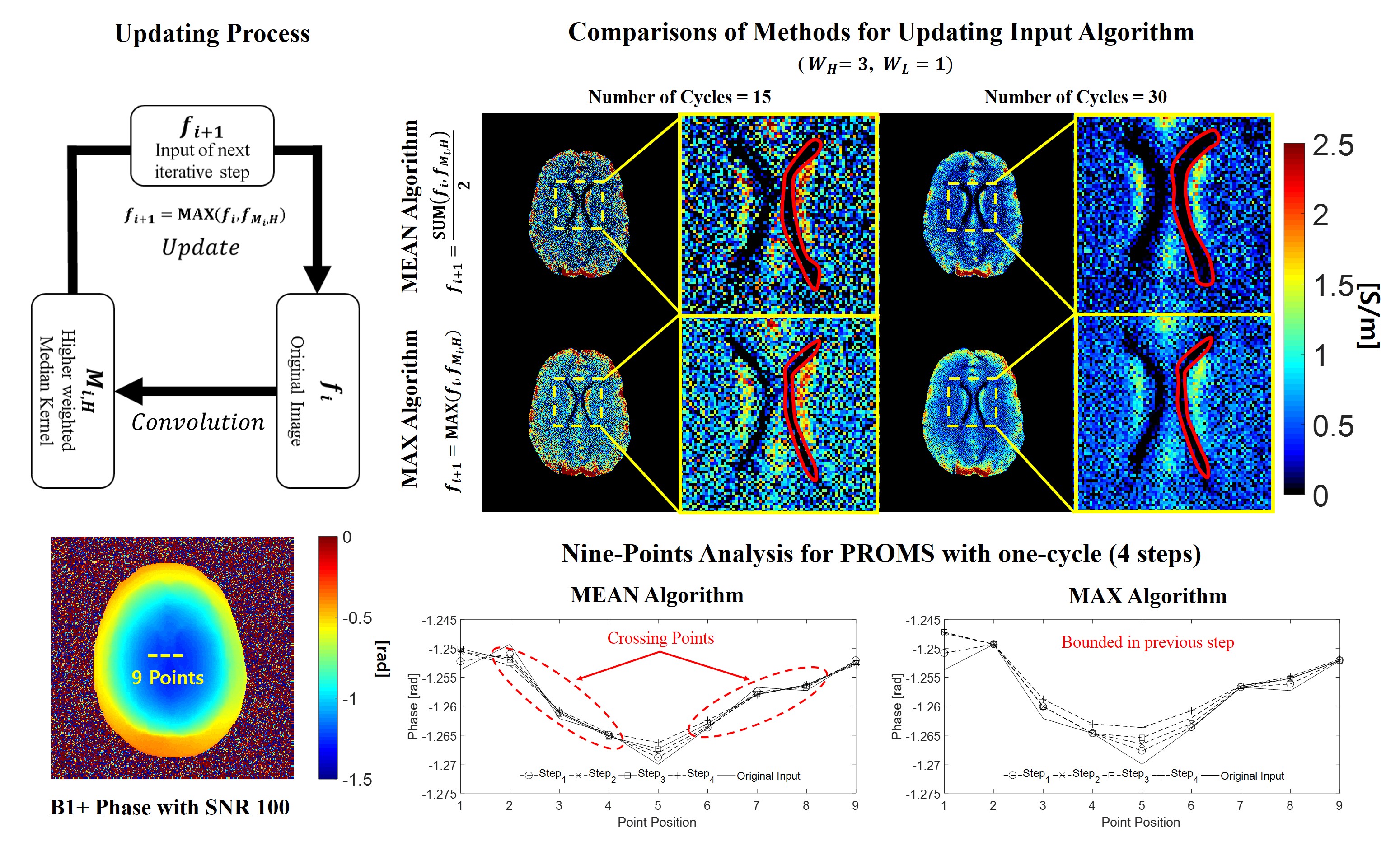
To prevent intensity loss near the boundary during iterative Median projections, the input is updated by using the MAX operator. The input for the next iterative step can be expressed as:
$$f_{i+1}=MAX[f_{i},\hat{f_{H}}],$$
where the input is convolved with a high weighting Median kernel, $$$\hat{f_{H}}=f_{i}*M_{i,H}$$$.
From here, each values of pixels in the input is bounded in the previous iterative step and it will protect intensity loss near the boundary in iterative Median projections. It means that increase of conductivity with negative values, which is known as boundary artifacts, are blocked during the update process.The proposed processing scheme is explained in Fig. 1.
3. EPT Reconstruction
The phase-based electrical conductivity reconstruction can be simplified as 7:
$$\sigma\approx\frac{\triangledown^{2}\phi_{0}}{2\omega\mu_{0}}$$
where $$$\phi_{0}$$$, $$$\omega$$$, and $$$\mu_{0}$$$ denote transceiver phase, Larmor frequency in Rad/sec, and the magnetic permeability, respectively.
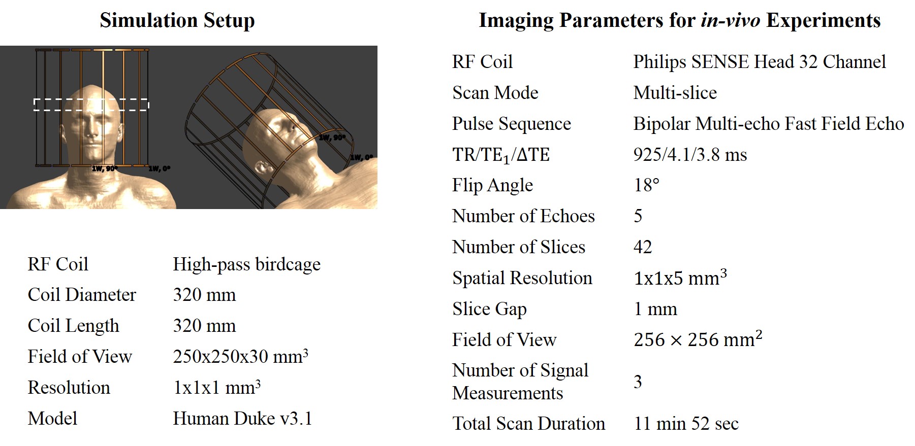
4. Data Acquisition
For validation of the proposed method, FDTD simulations were conducted using Sim4Life (ZMT AG, Zurich, CH)8.
In-vivo experiments were performed on 3.0T MRI system (Philips Achieva, The Netherlands). For reproducibility test, three healthy volunteers were scanned using multiple gradient-echo sequence and the transceiver phase was estimated using the linear fitting method.9
Detailed imaging parameters are shown in Fig.2.
Results
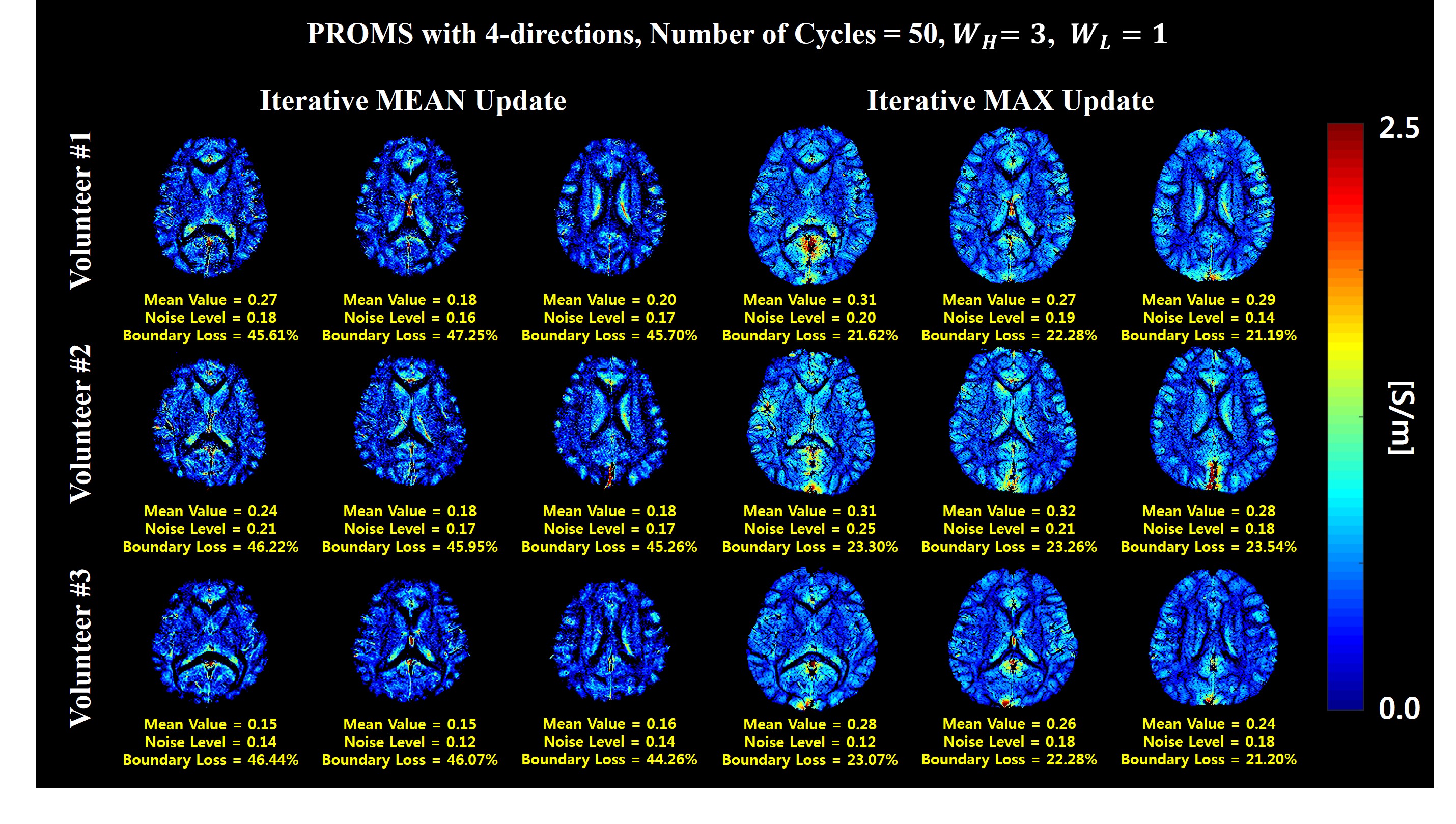
The simulation results using two updating methods for PROMS are compared in Fig. 3. The imaging result from MAX algorithm shows higher performance in SNR and better boundary definition in EPT than that from the MEAN algorithm and the size of boundary errors remains same as its initial state. This is because the MAX algorithm does not have zero crossing points as shown in the nine-point analysis results(Fig. 3).Conductivity maps obtained for three volunteers are shown in Fig. 4. The MEAN algorithm, whose results are similar with those obtained by using standard Laplacian with multi-stage denoising, has almost twice larger boundary errors and higher noise level than the MAX algorithm. However, flow artifacts were occured near the sinus when using MAX algorithm. This seems to be due to the nonlinear characteristics of flow artifacts due to unstable phase values.
Discussion and Conclusions
In this study, we proposed the novel method for estimating the Laplacian using projection onto Rotating Median sets. The advantages of the proposed method are summarized below:1. The proposed Median kernel sets can be implemented in Fourier domain resulting in fasten calculation time.
2. The degree of smoothing can be controlled by adjusting the center weight values, which results in better edge preserving.
3. In the updating process, MAX algorithm helps to keep the boundary loss in initial state.
However, more study is required to correct the initial boundary error and flow artifact.
Acknowledgements
This work was supported by the Technology Innovation Program (#10076675) funded by the Ministry of Trade, Industry Energy (MOTIE, Korea).References
1.Katscher U et al., Recent progress and future challenges in MR electric properties tomography. Comput Math Methods Med. 2013; 546-62.2. van Lier AL et al., B1(+) Phase Mapping at 7T and its Application for In Vivo Electrical Conductivity Mapping. Magn Reson Med. 2012; 67(2):552-61.
3. Hafalir FS et al., Convection-reaction equation based magnetic resonance electrical properties tomography (cr-MREPT). IEEE Trans Med Imaging 2014; 33(3):777-93.
4. Michel E et al., Electrical conductivity and permittivity maps of brain tissues derived from water content based on T1-weighted acquisition. Magn Reson Med. 2016; 77(3)
5. Gurler N et al., Gradient-based electrical conductivity imaging using MR phase. Magn Reson Med. 2017; 77(1):137-150.
6. Shin JW et al., Redesign of the Laplacian kernel for improvements in conductivity imaging using MRI. Magn Reson Med. 2018; Online version.
7. van Lier AL et al., Electrical properties tomography in the human brain at 1.5, 3. And 7T: a comparison study. Magn Reson Med. 2014; 71(1):354-63.
8. Sim4Life by ZMT, http://www.zurichmedtech.com
9. Kim DH et al., Simultaneous imaging of in vivo conductivity and susceptibility. Magn Reson Med. 2014; 71(3): 1144-50.
Figures