4627
3D Selective RF and Gradient Waveforms designed by using a GPU Accelerated Genetic Algorithm1Sir Peter Mansfield Imaging Centre, School of Physics & Astronomy, University of Nottingham, Nottingham, United Kingdom
Synopsis
The Genetic Algorithm (GA) is motivated by the process of natural selection, allowing mutliple initialisations. Due to the stochastic nature of genetic algorithms they are beneficial in avoiding local minima, although they can require significantly more function evaluations to run than a traditional solver. In this work, motivated by the field of shape optimisation, an approach is taken to perform the joint design of RF and gradient waveforms using a GA with a GPU-accelerated iterative solver.
Introduction
In certain applications, full three-dimensional (3D) spatial excitation is useful. The joint optimisation of both RF and gradient waveforms has been shown to reduce the excitation error in comparison to optimising RF pulses alone$$$^1$$$. Previous joint-methods$$$^{2,3}$$$ typically use local solvers that are susceptible to the initial conditions. The Genetic Algorithm (GA) is motivated by the process of natural selection, allowing mutliple initialisations. Due to the stochastic nature of genetic algorithms they are beneficial in avoiding local minima, although they can require significantly more function evaluations to run than a traditional solver. In this work, an optimisation approach is taken to perform the joint design of RF and gradient waveforms using a GA with a GPU-accelerated iterative solver.
Theory
The joint optimisation of RF$$$(\mathbf{b})$$$ and Gradient waveforms (represented by parameters $$$\rho$$$) over $$$N_t$$$ time points is formalised as:
$$\begin{split}\min_{\mathbf{b}\in\mathbb{C}^{N_tN_c},\rho^{3N_{\rho}}}\big\{||A(\rho)\mathbf{b}- &\mathbf{m}_{\text{target}}||^2+\lambda||\mathbf{b}||^2\big\}\\\text{s.t.}|\mathbf{G}_i[j]|&<\mathbf{G}_{\text{max}}\\|\Delta\mathbf{G}_i[j]|&< \mathbf{S}_{\text{max}}\Delta t\\\forall i\in\{x,y,z\},&j\in\{1,...,N_t\}\\\end{split}$$
where $$$A(\rho)$$$ represents the system encoding matrix including off-resonance effects, and $$$N_c$$$ coil-sensitivities. The 3D magnetisation target $$$\mathbf{m}_{\text{target}}$$$ consists of $$$N_s$$$ spatial voxels. The maximum gradient amplitude and slew rates are denoted by $$$\mathbf{G}_\text{max}$$$ and $$$\mathbf{S}_\text{max}$$$ respectively.
We parameterise the gradient waveforms as a linear transformation of $$$N_{\rho}$$$ parameters per axis, where $$$N_{\rho} \ll N_t$$$. As the gradients played out by the scanner hardware can be significantly distorted compared to the input waveforms; we convolve each basis function $$$g_k(t)$$$ with the associated Gradient Impulse Response Function$$$^5$$$ (GIRF) , $$$H(t)$$$ for each axis.
$$G_i(t)=\sum_{k=1}^{N_{\rho}}\rho_k^{(i)}\Big(H^{(i)}(t)*g_k(t)\Big)=\sum_{k=1}^{N_{\rho}}\rho_k^{(i)} \tilde{g}_k^{(i)}(t)$$
We can conveniently precompute the convoluted basis functions and rapidly calculate a new distorted gradient waveform by matrix multiplication.
Methods
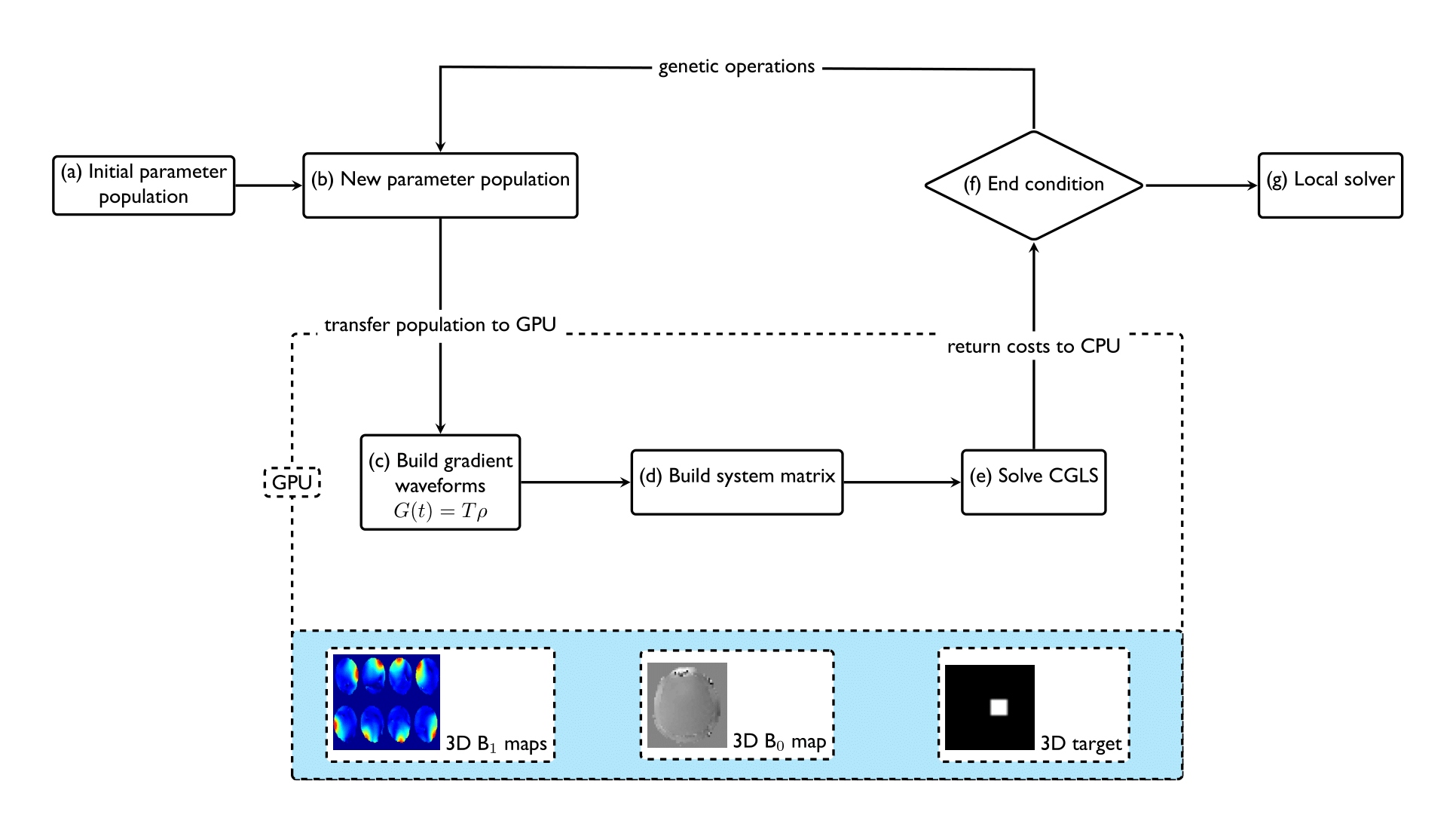
Equation 1 is cast as an alternating minimisation consisting of a GA outer loop for gradient parameters and a GPU-accelerated conjugate gradient least squares (CGLS) inner loop for RF pulses. 50 parameters per axis were used to define the gradient waveform shapes.To minimise data transfer across the CPU-GPU bridge, all $$$B_1^+$$$, $$$B_0$$$ maps, target profiles, and transformation matrices reside on the GPU in device memory. After each GA update, the new gradient parameters are transferred to the GPU and uncompressed (we used both linear piecewise and discrete cosine transformations (DCT)). The system matrix $$$A$$$ is calculated directly, including any off-resonance terms. We implemented a CGLS solver using high level MATLAB constructs directly on the GPU. CGLS is dominated by two matrix multiplications $$$m=Ab$$$ and $$$b=A^Hp$$$ which are well suited for parallelisation. Only the residual error is returned to the CPU to be used in the next genetic update. An NVIDIA Titan X GPU was used for all work (28 streaming-multiprocessors; 12Gb memory).
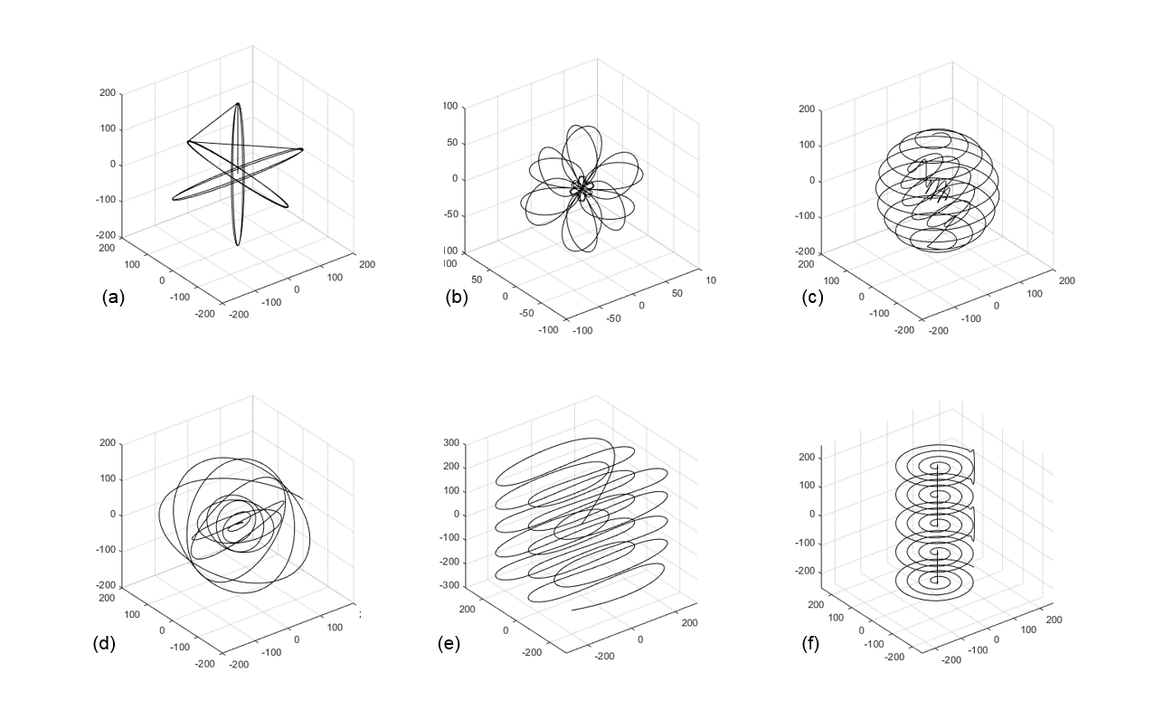
The GA was seeded with an initial population of 100 randomly drawn parameter sets and 100 scaled versions of several "classic" trajectories including: Shells$$$^6$$$; extended SPINS$$$^7$$$; EVI$$$^8$$$; stack-of-spirals$$$^9$$$ extended kT-points$$$^{6,10}$$$; cross$$$^{3}$$$; "petal" - a rosette like trajectory$$$^{11}$$$ (see Figure 2). Gradient waveforms for each of the trajectories were generated using the time-optimal method$$$^{12}$$$ and accordingly adjusted to a duration of 6.4ms at a resolution of 6.4$$$\mu$$$s. The maximum allowed gradient amplitude tolerated was limited to 40mTm$$$^{-1}$$$, and maximum allowed slew rate was 150Tm$$$^{-1}$$$s$$$^{-1}$$$.
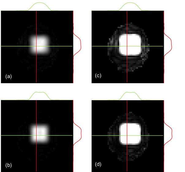
Bloch simulations were used to validate the performance of the designed waveforms using experimentally-acquired field maps (Nova Medical 8Tx/32Rx head-only RF coil). Two seperate 3D transverse magnetisation targets were defined: a cube of dimension (10cm$$$^3$$$), and a cuboid (5,20,7.5)cm. A local solver was also evaluated using the interior-point algorithm along with the best initial starting point in each case.
Results
Optimisation reduced the excitation error in all cases. Although for interior-point solver this improvement was marginal at less than 5%, but converged in under 10 minutes. Extended-SPINS had the lowest error from the initial population of k-space trajectories for both magnetisation targets. The GA yielded a reduced target error of between 20-30% over the interior-point solver, at the expense of a much greater computational time (this was manually terminated at 1 hour). Parameterisation using a DCT achieved a lower ($$$\approx$$$30% reduced) error than the piecewise transformation for the same number of parameters in all cases. There was less than a negligible change in transmit power between the methods.Discussion
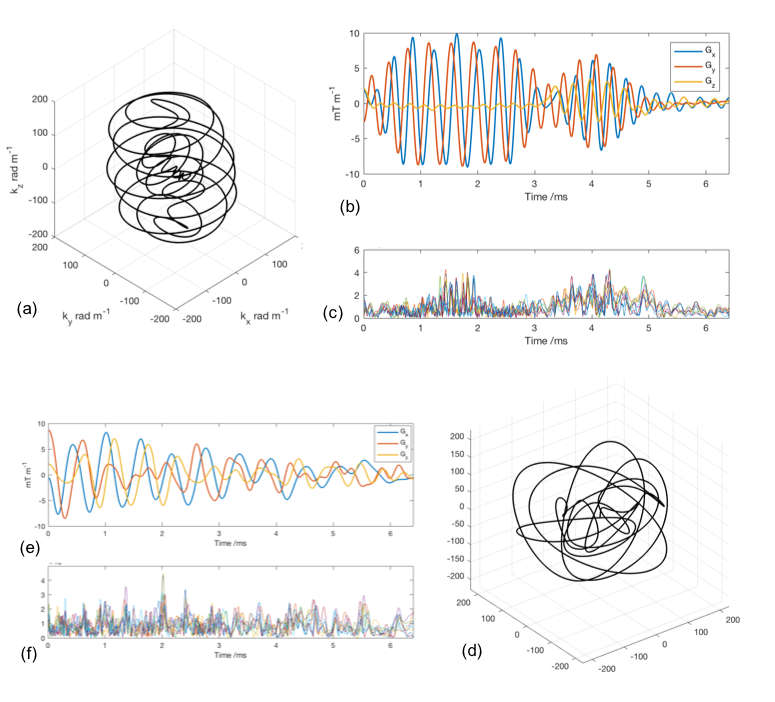
The actual trajectories designed for each target are visually quite different (see Figure 4). For a cubic target a modified shells trajectory (highly undersampled) is observed, where as for the cuboidal target the $$$k_z$$$ extent of the trajectory noticeably reduced. We cannot claim either of these are the global solution due the stochastic nature of the GA, although the the excitations profiles are cleaner.The DCT was able to achieve lower target error in all cases, suggesting it is a useful parameterisation in these cases. Despite the use of GPUs in this work, another order-of-magnitude speedup is required for online use and experimental validation.Acknowledgements
This work was supported by funding from the Engineering and Physical Sciences Research Council (EPSRC) and Medical Research Council (MRC) [grant number EP/L016052/1]. We gratefully acknowledge the support of NVIDIA Corporation with the donation of the Titan X Pascal GPU used for this research.References
[1]. Schneider JT, Kalayciyan R, Haas M, Herrmann SR, RuhmW, Hennig J, et al. Inner-volume imaging in vivo using threedimensionalparallel spatially selective excitation. Magnetic Resonance in Medicine 2013.
[2]. Hao S, Fessler JA, Noll DC, Nielsen JF. Joint design of excitation k-space trajectory and RF pulse for small-tip 3D tailoredexcitation in MRI. IEEE Transactions on Medical Imaging 2016;35(2):468–479.
[3]. Davids M, Schad LR,Wald LL, Guérin B. Fast three-dimensional inner volume excitations using parallel transmission andoptimized k-space trajectories. Magnetic Resonance in Medicine 2016;.
[4]. Yip CY, Grissom WA, Fessler JA, Noll DC. Joint design of trajectory and RF pulses for parallel excitation. MagneticResonance in Medicine 2007;58(3):598–604.
[5]. Vannesjo SJ, Haeberlin M, Kasper L, Pavan M, Wilm BJ, Barmet C, et al. Gradient system characterization by impulseresponse measurements with a dynamic field camera. Magnetic Resonance in Medicine 2013;.
[6]. Wong STS, Roos MS. A strategy for sampling on a sphere applied to 3D selective RF pulse design. Magnetic Resonancein Medicine 1994;32:778–784.
[7]. Malik SJ, Keihaninejad S, Hammers A, Hajnal JV. Tailored excitation in 3D with spiral nonselective (SPINS) RF pulses.Magnetic Resonance in Medicine 2012;67(5):1303–1315.
[8]. Mansfield P. Multi-planar image formation using NMR spin echoes. Journal of Physics C: Solid State Physics1977;10:L55–L58.
[9]. Pauly JM, Hu BS, Wang SJ, Nishimura DG, Macovski A. A three-dimensional spin-echo or inversion pulse. MagneticResonance in Medicine 1993;29(1):2–6.
[10]. Chen D, Bornemann F, Vogel M, Sacolick L, Kudielka G, Zhu Y. Sparse Parallel Transmit Pulse Design Using OrthogonalMatching Pursuit Method. In: Proceedings 17th Scientific Meeting, International Society for Magnetic Resonance inMedicine, Honolulu; 2009. p. 171.
[11]. Noll DC. Multishot rosette trajectories for spectrally selective mr imaging. IEEE Transactions on Medical Imaging 1997.
[12]. Lustig M, Kim SJ, Pauly JM. A fast method for designing time-optimal gradient waveforms for arbitrary k-space trajectories.IEEE Transactions on Medical Imaging 2008;.
Figures