4403
Myelin Water Fraction Estimation using Small-Tip Fast Recovery MRI1Electrical Engineering and Computer Science, University of Michigan, Ann Arbor, MI, United States, 2Radiology, Memorial Sloan Kettering Cancer Center, New York, NY, United States, 3Biomedical Engineering, University of Michigan, Ann Arbor, MI, United States
Synopsis
Myelin water fraction (MWF) is a good biomarker for myelin content. Traditional methods for acquiring MWF maps require long scan times. Recent work has estimated MWF from faster steady-state scans. In this work, we propose to acquire MWF maps from an optimized set of small-tip fast recovery (STFR) scans that can exploit resonance frequency differences between myelin water and the slow-relaxing water compartment.
Introduction
Myelin water fraction (MWF), the proportion of MR signal in a given voxel that originates in water bound within the myelin sheath, is a specific biomarker for myelin content. Such a biomarker is desirable for tracking the onset and progression of demyelinating diseases such as multiple sclerosis. A common way to estimate MWF is from a multi-echo spin echo (MESE) pulse sequence, which is time-consuming.1 Recent work has estimated MWF from fast steady-state sequences.2 In this abstract, we propose estimating MWF from an optimized set of small-tip fast recovery (STFR) scans that can exploit resonance frequency differences between myelin water and the slow-relaxing water compartment. Simulation results illustrate how well STFR scans can estimate MWF.
Methods
The STFR pulse sequence3 consists of a tip-down RF pulse, signal readout, a tip-up RF pulse, and a spoiler gradient. The transverse signal generated by a single STFR scan at a particular voxel (for a single compartment) is
$$M_T\left(M_0,T_1,T_2,\Delta\omega,\kappa,T_{\mathrm{free}},T_{\mathrm{g}},\alpha,\beta,\phi\right) = \frac{M_0 \sin\left(\kappa\cdot\alpha\right)\left[e^{-T_{\mathrm{g}}/T_1}\left(1-e^{-T_{\mathrm{free}}/T_1}\right)\cos\left(\kappa\cdot\beta\right)+\left(1-e^{-T_{\mathrm{g}}/T_1}\right)\right]}{1-e^{-T_{\mathrm{g}}/T_1}e^{-T_{\mathrm{free}}/T_2}\sin\left(\kappa\cdot\alpha\right)\sin\left(\kappa\cdot\beta\right)\cos\left(\Delta\omega\cdot T_{\mathrm{free}}-\phi\right)-e^{-T_{\mathrm{g}}/T_1}e^{-T_{\mathrm{free}}/T_1}\cos\left(\kappa\cdot\alpha\right)\cos\left(\kappa\cdot\beta\right)},$$
where $$$M_0$$$ is proton density, $$$T_1$$$ is the spin-lattice relaxation time constant, $$$T_2$$$ is the spin-spin relaxation time constant, $$$\Delta\omega$$$ is off-resonance frequency, $$$\kappa$$$ is a flip angle scaling factor (to account for imperfect transmit fields), $$$T_{\mathrm{free}}$$$ is the time between the tip-down and tip-up pulses, $$$T_{\mathrm{g}}$$$ is the duration of the spoiler gradient, $$$\alpha$$$ is the prescribed tip-down flip angle, $$$\beta$$$ is the prescribed tip-up flip angle, and $$$\phi$$$ is the phase of the tip-up pulse. Note that $$$M_0$$$, $$$T_1$$$, $$$T_2$$$, $$$\Delta\omega$$$, and $$$\kappa$$$ vary from voxel to voxel, whereas $$$T_{\mathrm{free}}$$$, $$$T_{\mathrm{g}}$$$, $$$\alpha$$$, $$$\beta$$$, and $$$\phi$$$ are scan parameters that are prescribed over the whole imaging volume.
We consider two non-exchanging intra-voxel water compartments: a fast-relaxing compartment with relaxation time constants $$$T_{1,\mathrm{f}}$$$ and $$$T_{2,\mathrm{f}}$$$, and a slow-relaxing compartment with relaxation time constants $$$T_{1,\mathrm{s}}$$$ and $$$T_{2,\mathrm{s}}$$$. We assume the fast-relaxing compartment experiences an additional off-resonance shift $$$\Delta\omega_\mathrm{f}$$$.4 The signal from a given voxel is a weighted sum of the signal that arises from the fast-relaxing and slow-relaxing compartments, where the weights are $$$f_\mathrm{f}$$$ and $$$1 - f_\mathrm{f}$$$, respectively, and $$$f_\mathrm{f}$$$ denotes the fraction of the signal arising from the fast-relaxing compartment. We estimate the MWF $$$f_\mathrm{f}$$$ for each voxel from multiple STFR scans.
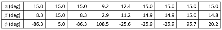
We optimized a set of 9 STFR scans to maximize the precision of estimates of $$$f_\mathrm{f}$$$. We minimized the expected Cramer-Rao Bound (CRB) of estimates of $$$f_\mathrm{f}$$$.5 We fixed $$$T_{\mathrm{free}}$$$ to 8.0 ms and $$$T_{\mathrm{g}}$$$ to 1.5 ms and optimized $$$\alpha$$$, $$$\beta$$$, and $$$\phi$$$. For $$$\Delta\omega$$$ and $$$\kappa$$$ we used separately acquired B0 and B1 maps, respectively. Table 1 lists the optimized scan parameters.
Using the optimized scan parameters, we simulated the 9 STFR scans using a slice of the BrainWeb phantom.6 For white matter, we assigned $$$M_0 = 0.77$$$, $$$f_\mathrm{f} = 0.15$$$, $$$T_{1,\mathrm{f}} = T_{1,\mathrm{s}} = 832$$$ ms, $$$T_{2,\mathrm{f}} = 20$$$ ms, $$$T_{2,\mathrm{s}} = 80$$$ ms, and $$$\Delta\omega_\mathrm{f} = 17$$$ Hz; and for gray matter, we assigned $$$M_0 = 0.86$$$, $$$f_\mathrm{f} = 0.03$$$, $$$T_{1,\mathrm{f}} = T_{1,\mathrm{s}} = 1331$$$ ms, $$$T_{2,\mathrm{f}} = 20$$$ ms, $$$T_{2,\mathrm{s}} = 80$$$ ms, and $$$\Delta\omega_\mathrm{f} = 0$$$.2 We generated $$$\kappa$$$ to vary from 0.8 to 1.2 (i.e., 20% flip angle variation), and $$$\Delta\omega$$$ to vary from -20 to 20 Hz. We added complex Gaussian noise to produce images with SNR ranging from 89-244 in white matter and 64-236 in gray matter, where SNR is defined as $$$\mathrm{SNR}\left(\mathbf{y},\boldsymbol{\epsilon}\right) \triangleq \frac{\|\mathbf{y}\|_2}{\|\boldsymbol{\epsilon}\|_2}$$$, where $$$\mathbf{y}$$$ is the noiseless data within a region of interest (ROI), and $$$\boldsymbol{\epsilon}$$$ is the noise added to the ROI. We estimated $$$f_\mathrm{f}$$$ from the STFR images using kernel machine learning.7
Results
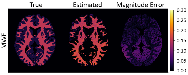
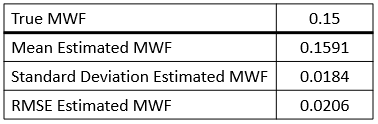
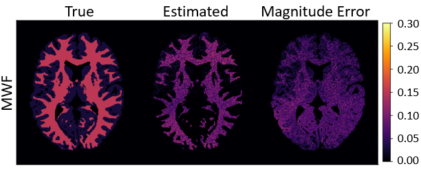
Figure 1 compares the $$$f_\mathrm{f}$$$ estimates from the simulated STFR scans to the true values of $$$f_\mathrm{f}$$$. Table 2 reports sample statistics of the $$$f_\mathrm{f}$$$ estimates. Interestingly, $$$f_\mathrm{f}$$$ is estimated accurately in white matter voxels (where $$$\Delta\omega_\mathrm{f} = 17$$$ Hz), but not in gray matter voxels (where $$$\Delta\omega_\mathrm{f} = 0$$$, i.e., both the fast-relaxing and slow-relaxing compartments experience the same off-resonance frequency). Figure 2 is the same as Figure 1, except now $$$\Delta\omega_\mathrm{f} = 0$$$ everywhere. In this case, estimates of $$$f_\mathrm{f}$$$ in white matter are also inaccurate.Discussion and Conclusion
From simulation, we see that optimized STFR scans can accurately and precisely estimate MWF in white matter. It is also clear that STFR exploits the difference between the off-resonance frequency experienced by the slow- and fast-relaxing compartments; the smaller the difference is, the worse the estimates of $$$f_\mathrm{f}$$$ are. In this simulation, a constant $$$\Delta\omega_\mathrm{f}$$$ was simulated for all white matter voxels; future work will consider $$$\Delta\omega_\mathrm{f}$$$ variations throughout white matter.4Acknowledgements
No acknowledgement found.References
[1] A. Mackay, K. Whittall, J. Adler, D. Li, D. Paty, and D. Graeb. In vivo visualization of myelin water in brain by magnetic resonance. Mag. Res. Med., 31(6):673–7, June 1994.
[2] G. Nataraj, J-F. Nielsen, M. Gao, J. A. Fessler. Fast, precise myelin water quantification using DESS MRI and kernel learning. arXiv:1809.08908v1 [physics.med-ph].
[3] J-F. Nielsen, D. Yoon, D. Noll. Small‐tip fast recovery imaging using non‐slice‐selective tailored tip‐up pulses and radiofrequency‐spoiling. Mag. Res. Med., 69(3):657-66, March 2013.
[4] K. Miller, S. Smith, P. Jezzard. Asymmetries of the balanced SSFP profile. Part II: white matter. Mag. Res. Med., 63(2):396-406, February 2010.
[5] G. Nataraj, J-F. Nielsen, and J. A. Fessler. Optimizing MR scan design for model-based T1, T2 estimation from steady-state sequences. IEEE Trans. Med. Imag., 36(2):467–77, February 2017.
[6] D. L. Collins, A. P. Zijdenbos, V. Kollokian, J. G. Sled, N. J. Kabani, C. J. Holmes, and A. C. Evans. Design and construction of a realistic digital brain phantom. IEEE Trans. Med. Imag., 17(3):463–8, June 1998.
[7] G. Nataraj, J-F. Nielsen, C. D. Scott, and J. A. Fessler. Dictionary-free MRI PERK: Parameter estimation via regression with kernels. IEEE Trans. Med. Imag., 37(9):2103–14, September 2018.
Figures