4384
multiMap: A Gradient Spoiled Sequence for Quantitation of B1, B0, T1, T2, T2*, and Fat Fraction1Electrical Engineering, Stanford University, Stanford, CA, United States, 2Stanford Center for Cognitive and Neurobiological Imaging, Stanford University, Stanford, CA, United States, 3Biomedical Engineering, Northwestern University, Evanston, IL, United States
Synopsis
multiMap is a single sequence that combines standard techniques for measuring several quantities of interest: B0, B1, T1, T2, T2*, and Fat Fraction.
Introduction
The multiMap sequence combines several standard techniques for quantitative imaging into a single scan. The Saturated Double Angle Method (SDAM) of B1+ mapping [1] is an efficient method for making a B1 map of a volume. A saturation pulse is followed by some time for recovery before an imaging radio frequency (RF) pulse is emitted. The sequence is repeated for two imaging RF pulses of different flip angles ($$$60^\circ$$$ and $$$120^\circ$$$) from which the Double Angle Method of B1 mapping can be performed \cite{insko1993mapping}. When imaging a single slice, the recovery time after the saturation pulse and any time after the imaging pulse before recovery are dead time (i.e., the time is not used to gather relevant information). Here, we propose to fill this time with acquisitions to perform additional quantification. multiMap is a modification of SDAM when imaging one slice to simultaneously perform B1+ and B0 mapping; M0/T1, T2, and T2$$$^\ast$$$ quantification; and determine the fat fraction.
Methods
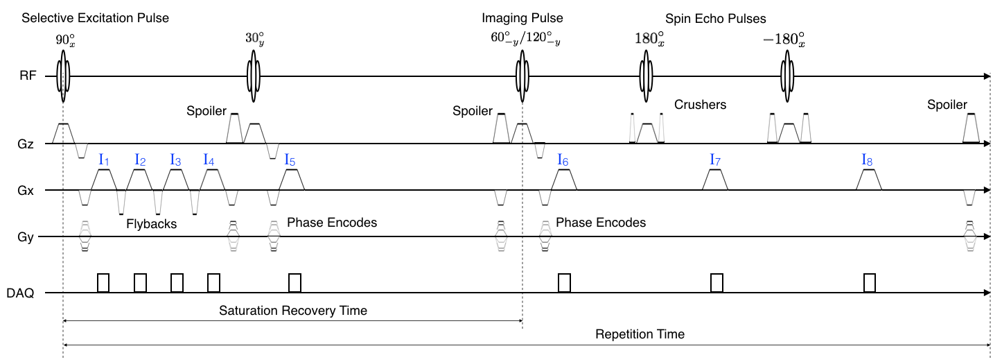
The complete Multi-Map sequence is shown in figure1. A two-dimensional Cartesian trajectory is used for acquisition. The saturation pulse is followed by four separate readout gradient waveforms interleaved with flyback gradient waveforms. The entire repetition is repeated twice (two segments): once with a flip angle of the 3rd RF pulse equal to $$$60^\circ$$$ and a second time with a flip angle of $$$120^\circ$$$. Sixteen separate images are acquired from which the quantitative maps are determined; the acquisition associated with the $$$j^{\text{th}}$$$ image is labeled in blue in figure 1.Images $$$I_6$$$ from both segments are used to quantify the $B_1$ map. If we assume that the saturation pulse works perfectly, then there is no residual $$$M_z$$$ from a previous acquisition. The $$$M_z$$$ component then recovers during saturation. The $$$30^\circ$$$ RF pulse that occurs during the saturation recovery time happens to both segments, so the $$$M_z$$$ at the end of the recovery time will be identical for both segments. Any remaining transverse magnetization is approximately eliminated by the spoiler at the end of the saturation recovery time. The flip angle can then be calculated according to the double angle formula [2]: $$$\alpha=\text{acos}\left( \sin(2\alpha) / 2\sin(\alpha) \right)$$$. Off resonance, T2$$$^{\ast}$$$, water, and fat are determined (similar to [3]) by solving the following optimization problem: $$$\text{minimize}\hspace{4pt}\|(I_1,I_2,I_3,I_4)-\hat{I}\|_2$$$, where
$$\hat{I_j} = e^{i\Delta\omega_0 t_j}\left[W + F \exp\left(i\Delta\omega_{cs} t_j\right) \right]e^{-t_j/T2}.$$
Here, $$$t_j$$$ is the time associates with images $$$I_j$$$; $$$W,F\in\mathbb{C}$$$; and $$$\omega_{cs}$$$ is the chemical shift frequency of fat. The fat fraction is $$$f_f=|F|/(|W|+|F|)$$$. T2 is estimated by fitting an exponential decay to the spin echo images $$$I_6-I_8$$$. The size of recovery duration saturation can be used to quantify T1. Two RF pulses are used to probe this state: a $$$30^\circ$$$ RF pulse after the fourth acquisition, and the $$$60^\circ$$$ RF pulse. A small $$$30^\circ$$$ pulse is used to yield measurable signal while leaving the amount of recovery relatively undisturbed. Images $$$I_5,I_6$$$ are used to quantify $$$M_0/T1$$$. Note that $$$M_z(t)=M_z(t_0)+M_0\left(1-\exp(-t/T1)\right)$$$. After saturation, $$$M_z=0$$$. Therefore, $$$M_z(t)\approx(M_0/T1)t$$$. By fitting a line to $$$|I_5|,|I_6|$$$,
$$ \frac{M_0}{T_1}\approx\frac{|I_6|-|I_5|}{t_6-t_5}. $$
$$$M_0$$$ and $$$T_1$$$ can be quantified independently by extending the saturation recovery time and fitting and exponential to the recovery (rather than a line).
Results
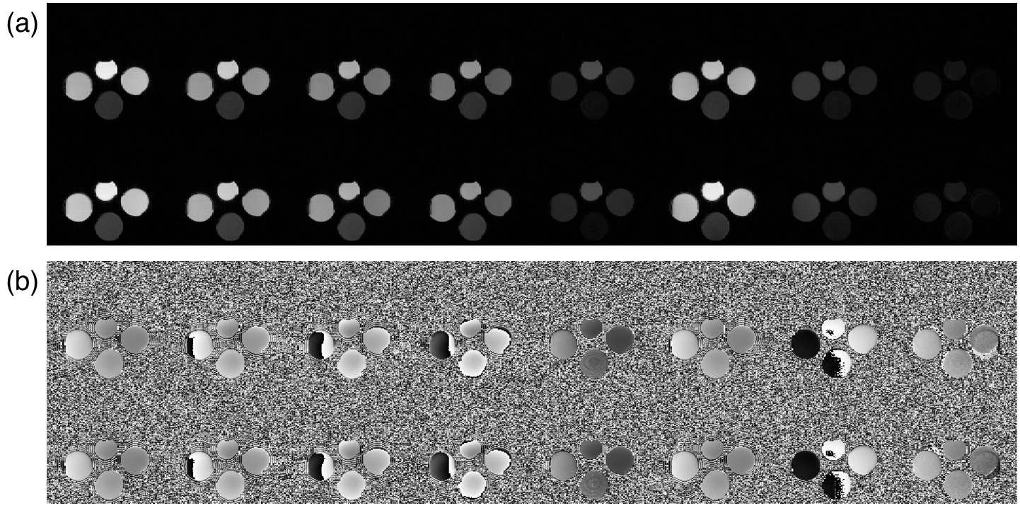
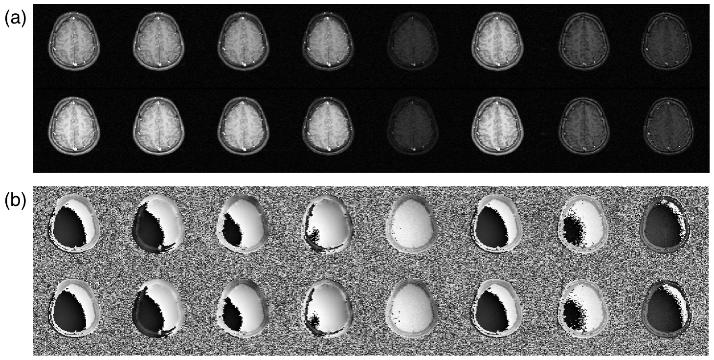
Results were generated with a 1.5 T commercial scanner and a $$$62.5$$$ kHz reception bandwidth. The repetition time was $$$400$$$ ms and the saturation recovery time was $$$200$$$ ms. RF chopping (alternating the phase of successive phase encode acquisitions by $$$\pi$$$) is used to push the majority of the zipper artifact to the image's edge.
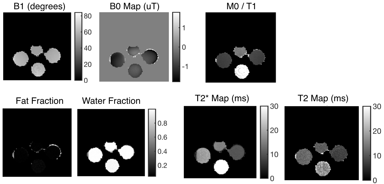
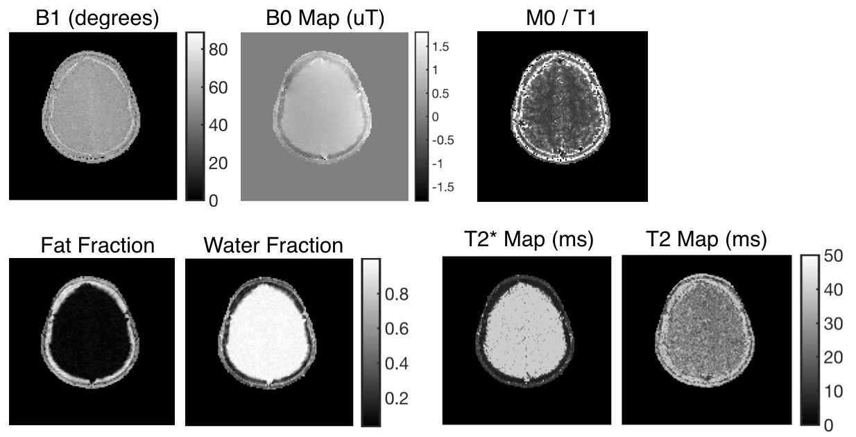
Two subject types were scanned: a set of bottles with varying T1s and T2s, and a slice of a brain. The reconstructions of the bottles and brain are shown in figures 2 and 4, respectively. The quantitative maps are shown in figures 3 and 5, respectively.
Conclusion
This abstract presents multiMap, a single sequence that generates many different quantitative maps. There are a large number of further improvements that could be made to this sequence. The Cartesian acquisition can be replaced with a spiral acquisition for reduced number of readouts (and a reduced total scan time). Additionally, the RF pulses and acquisitions of multiple slices can be interleaved to increase the volume of coverage. Finally, susceptibility can be quantified using the B0 map.Acknowledgements
No acknowledgement found.References
[1] Charles H Cunningham, John M Pauly, and Krishna S Nayak. Saturated double-angle method for rapidB1+ mapping.Magnetic Resonance in Medicine, 55(6):1326–1333, 2006.
[2] EK Insko and L Bolinger. Mapping of the radiofrequency field.Journal of Magnetic Resonance, Series A,103(1):82–85, 1993.
[3] Scott B Reeder, Zhifei Wen, Huanzhou Yu, Angel R Pineda, Garry E Gold, Michael Markl, and Norbert JPelc. Multicoil dixon chemical species separation with an iterative least-squares estimation method.Magnetic Resonance in Medicine: An Official Journal of the International Society for Magnetic Resonancein Medicine, 51(1):35–45, 2004.
Figures