4007
Accelerated Single-Min-Cut Graph-Cut Algorithm Using a Variable-Layer Graph Construction Improves Field-Mapping in Water–Fat Regions1Department of Diagnostic and Interventional Radiology, Technical University of Munich, Munich, Germany, 2Munich School of Bioengineering, Technical University of Munich, Munich, Germany
Synopsis
Accurate field-mapping is critical in body imaging for both robust water–fat separation and accurate quantitative susceptibility mapping. The present work proposes a single-min-cut field-mapping method to improve field-map results in water–fat regions. The proposed method based on a variable layer graph construction, solves the phase-wrapping problem and yields directly into non-wrapped field-maps. In challenging areas with low SNR or strongly varying field-maps the accuracy is significantly increased, while the computational cost is drastically reduced.
Introduction
Accurate $$$B_0$$$ field-mapping in body regions where water and fat components are present is required in order to perform both robust water–fat separation1 and accurate quantitative susceptibility mapping (QSM)2. Field-mapping in water–fat regions relies on optimizing the least square distance from multi gradient-echo images to a water–fat signal model, which is a non-convex optimization problem due to the non-linearity of the field-map term3. Different approaches have been proposed to solve the above problem by imposing a smoothness constraint on the field-map3,4. Algorithms formulating the problem as a graph search have been particularly successful in solving the constrained optimization problem using either min-cuts iteratively4 or single-min-cut approaches5,6 with however the drawback of long computational times. The present work proposes an accelerated single-min-cut graph cut algorithm for field-mapping in the presence of water-fat using a variable-layer graph construction.Methods
Theory
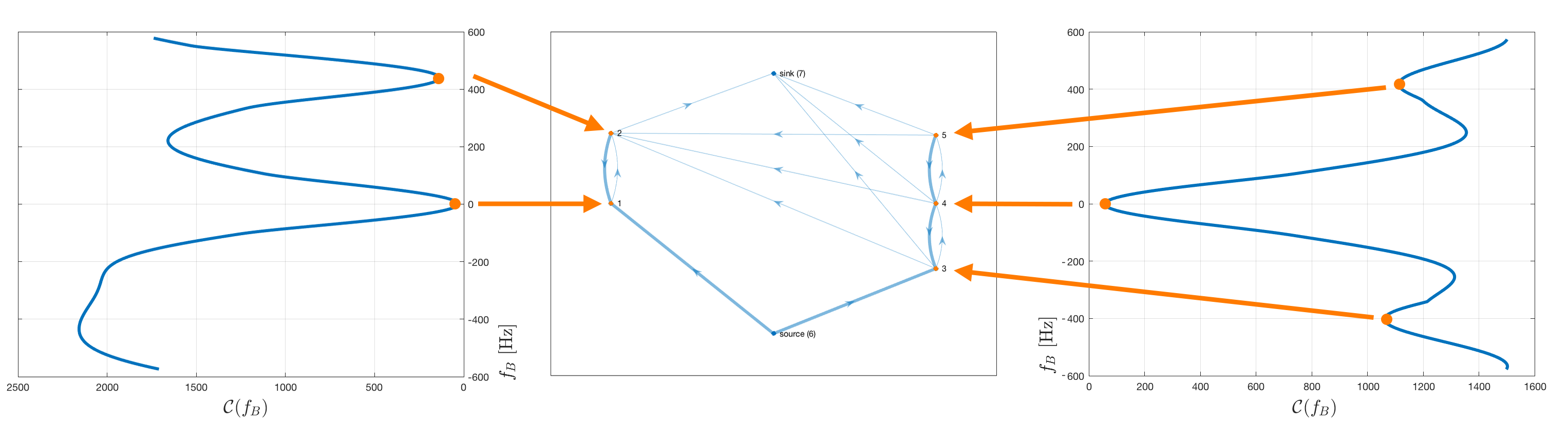
The VARPRO formulation is used to obtain voxel-wise field-map estimates $$$\mathcal{C}(f_B)$$$7 that account for the presence of fat, modeled with a 10-peak spectrum specific to bone marrow8 and a shared $$$R_2^*$$$-decay for water and fat. We propose a penalized maximum likelihood cost function, which allows to impose spatial smoothness and can be mapped into a graph cut problem9,10 solving the minimization $$\widehat{f_B}={\arg}\;{\underset{f_B(\mathbf{r})}{\min}}{\sum_{\mathbf{r}}}\left({\mathcal{C}(f_B(\mathbf{r}))}+{\sum_{\mathbf{s}{\in}N\mathbf(r)}}|f_B(\mathbf{r})-f_B(\mathbf{s})|^2\right),(1)$$ where $$$f_B(\mathbf{r})$$$ is the fieldmap and $$$\mathcal{C}(f_B(\mathbf{r}))$$$ is the least square data consistency term of the complex gradient echo data to a complex water–fat signal model, scaled to the interval $$$[0,1]$$$. At each voxel $$$\mathbf{r}$$$, fieldmap values are restricted to only local minimizers of $$$\mathcal{C}(f_B(\mathbf{r}))$$$. $$$N(r)$$$ is the voxel neighborhood, which was taken to be the 6-connected von Neumann neighborhood. The data consistency $$$\mathcal{C}(f_B(\mathbf{r}))$$$ is periodic with period $$$[-1/(2\Delta\textrm{TE}),1/(2\Delta\textrm{TE})]$$$ and can have varying number of local minimizers therein, which correspond to nodes in the graph. In contrast to previous methods, we not only restrict the nodes to only local minimizers, but also allow for a variable number of minimas (nodes) for each voxel $$$\mathbf{r}$$$ . This variable layer construction drastically reduces the number of edges in the graph.
Simulations
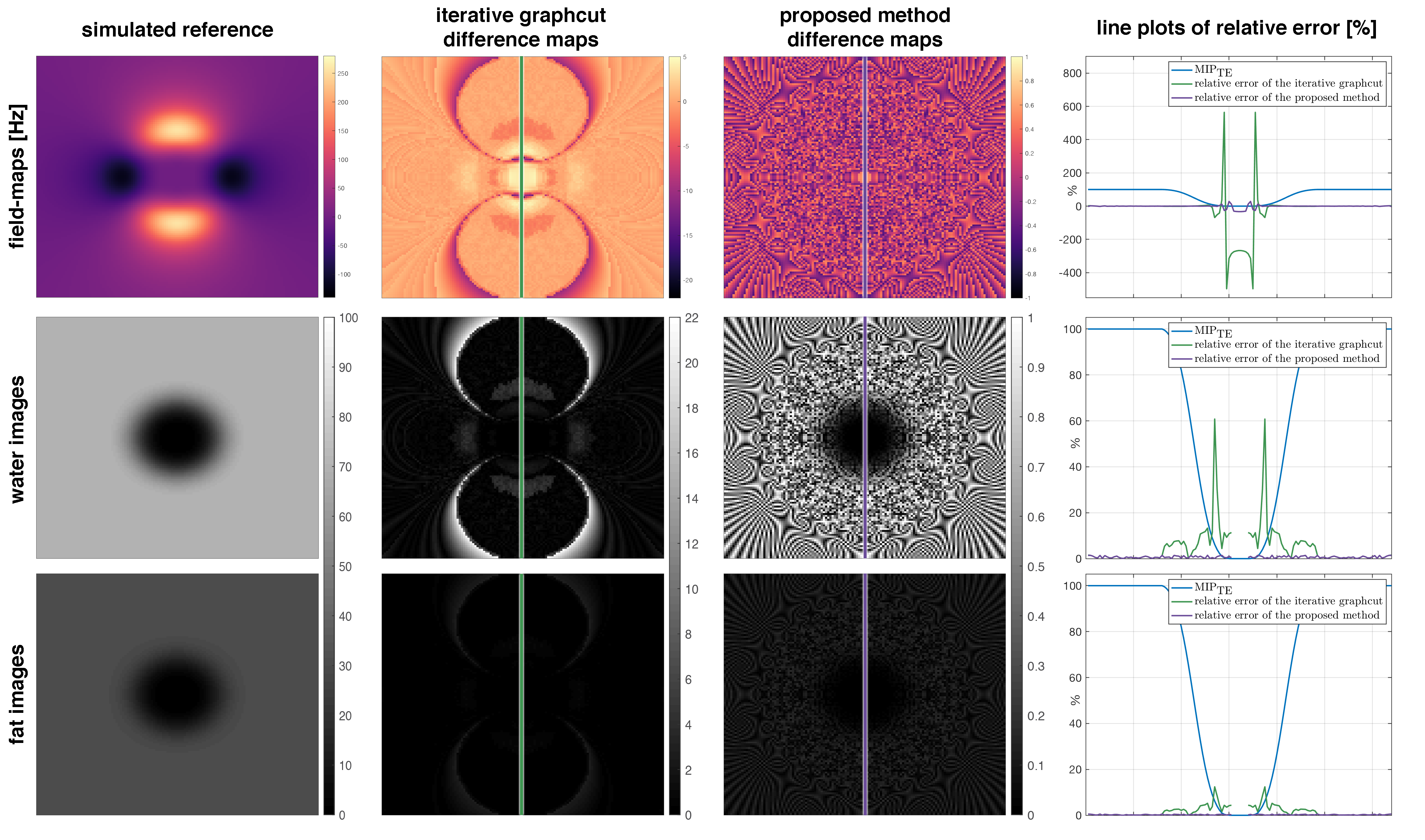
A numerical phantom with an air bubble in the center and surrounded by a fat fraction of 30$$$\:$$$% was set up. The interface from air to tissue was smoothed to have a continuous transition. Regions of air and different fat fractions were assigned their literature magnetic susceptibility values and a corresponding field-map was forward simulated.
In-vivo Measurements
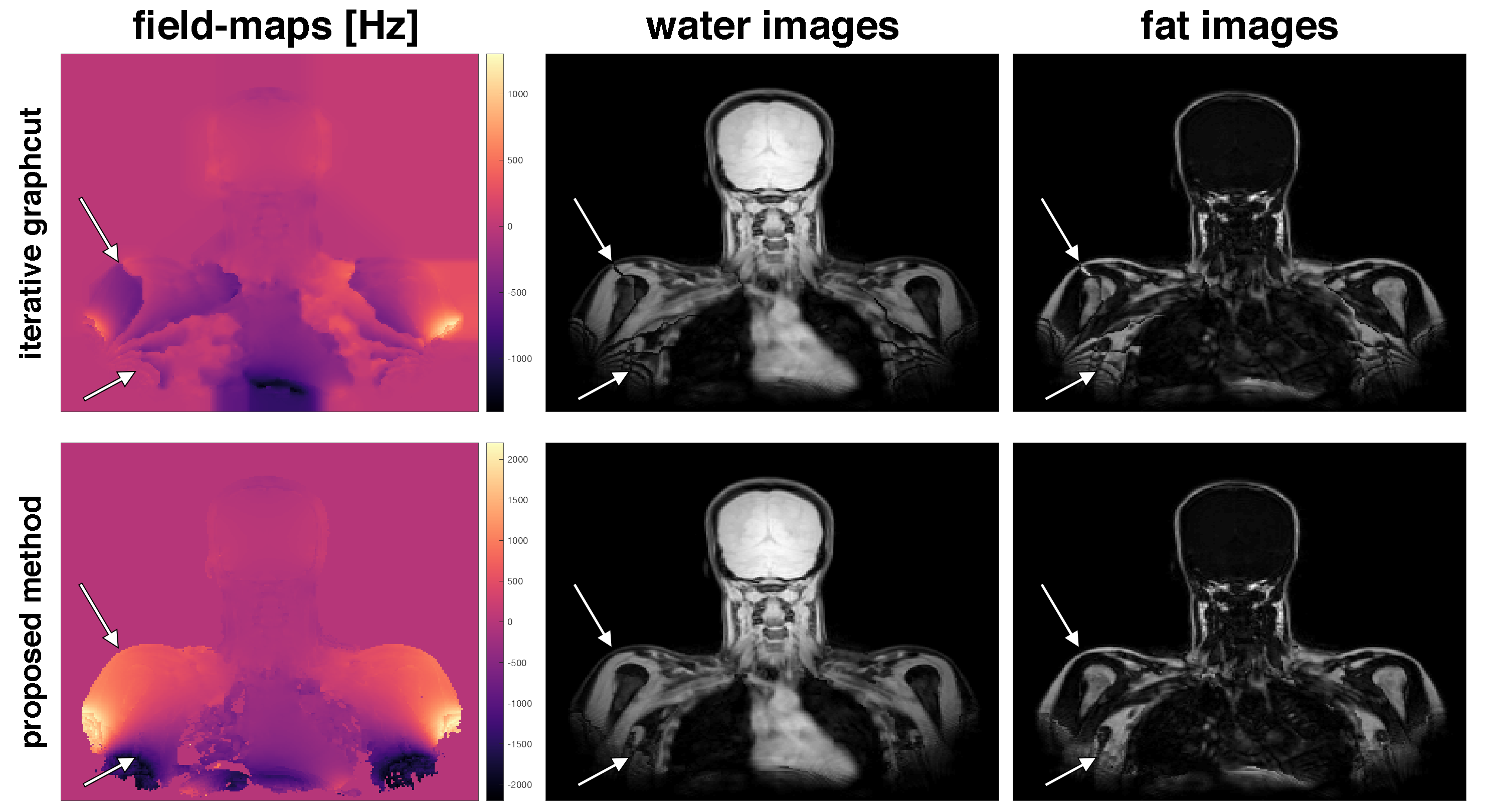
The method was applied to 3$$$\:$$$T datasets from a healthy cervical region and a pathological spine scanned with 3 and 6 echoes, respectively.
Comparison to Existing Methods
For both, simulation and in-vivo data, the proposed method was compared to a state-of-the-art iterative graph-cut algorithm4 and a recently proposed single-cut graph-cut algorithm6. In-vivo, a consistency check was performed by initializing a voxel-wise IDEAL algorithm11 with different graph-cut results to see whether the graph-cut results already converged to a true minimum of $$$\mathcal{C}(f_B(\mathbf{r}))$$$ in Equation (1).
Results
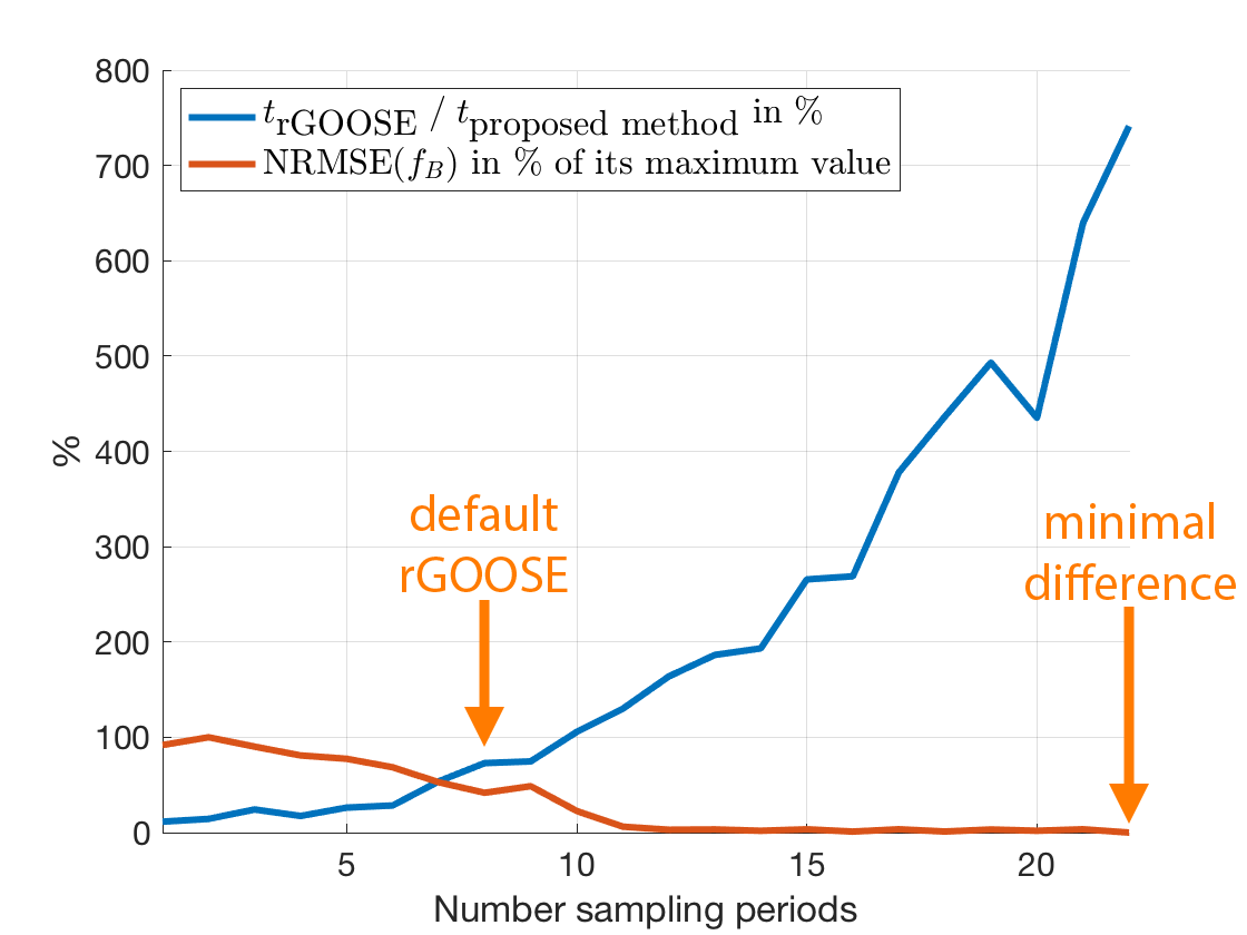
The proposed method efficiently addresses the issue that the number of minima varies from voxel to voxel. Therefore, the introduced variable-layer graph construction, illustrated in Figure 1, significantly reduces the size of the graph and significantly accelerates the computation compared to previously proposed single-min-cut graph-cut algorithms as shown in Figure 2.
Field-mapping in regions with strongly varying values can be greatly improved as shown in Figure 3 and the obtained field-maps are directly phase unwrapped as shown in Figure 4.
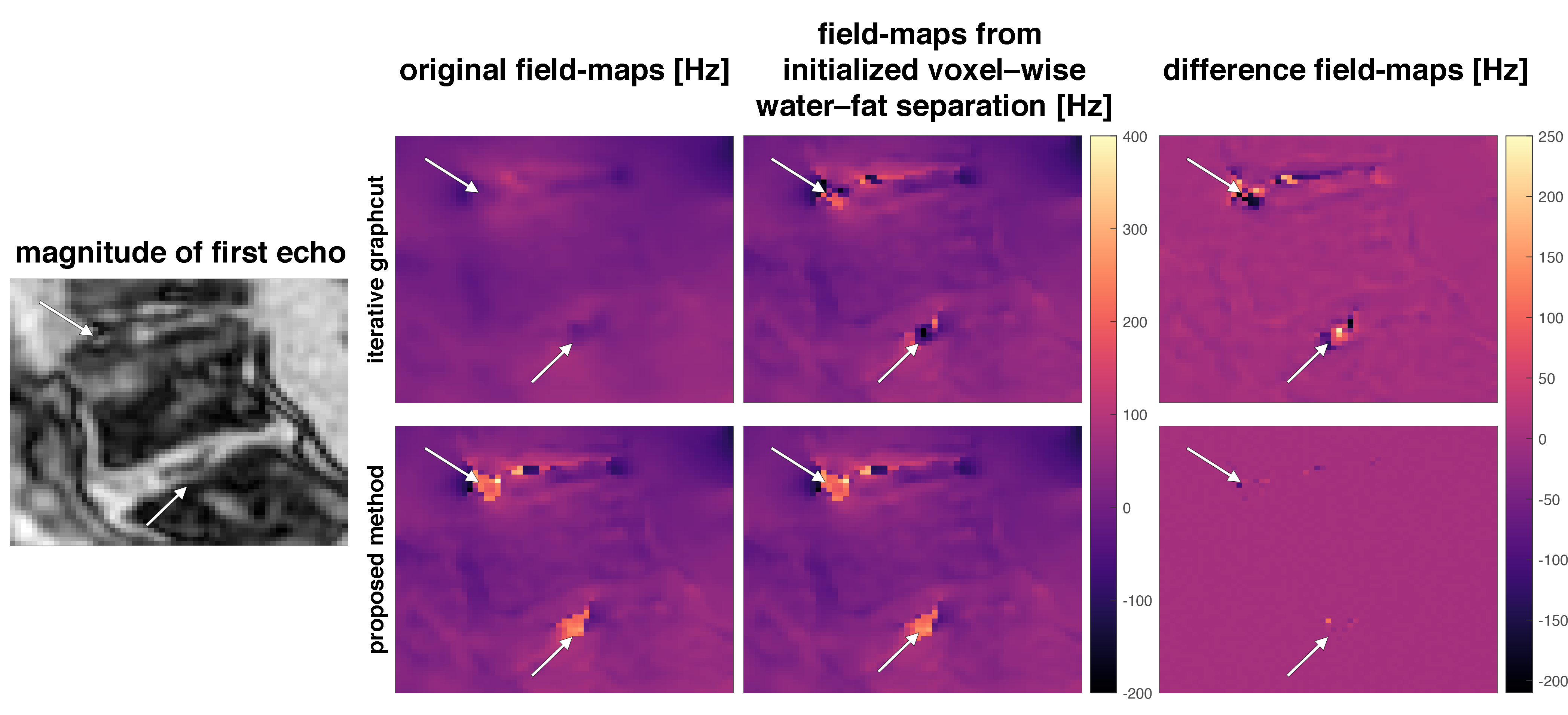
The proposed method yields meaningful field-map estimates in the borders of regions with low SNR and directly results in non-smoothed field-maps, like from a voxel-wise field-mapping method, as shown in Figure 5.
Discussion
The proposed method performs consistently better in regions with increased number of local minima in the field-map estimation due to either low SNR or rapidly varying field-maps. The proposed method yields directly phase-unwrapped field-maps. The obtained field-maps are non-smoothed like from a voxel-wise field-mapping method. Nevertheless, the proposed method is significantly faster than the previously proposed single-min-cut graph-cut method.
In conclusion, the proposed variable-layer graph-cut algorithm results in significantly lower computational cost due to the reduced graph size and more accurate field-map in regions with increased number of local minima.
Acknowledgements
The present work was supported by the European Research Council (grant agreement No.677661 – ProFatMRI). This work reflects only the authors view and the EU is not responsible for any use that may be made of the information it contains. The authors would also like to acknowledge research support from Philips Healthcare.
The software will be freely available at http://bmrrgroup.de/software/.
References
- Hu, H., Börnert, P., Hernando, D., Kellman, P., Ma, J., Reeder, S., Sirlin, C., ISMRM workshop on fat–water separation: Insights, applications and progress in MRI, Magnetic Resonance in Medicine, 68(2), (2012), http://dx.doi.org/10.1002/mrm.24369
- Wang, Y., Liu, T., Quantitative susceptibility mapping (QSM): Decoding MRI data for a tissue magnetic biomarker, Magnetic Resonance in Medicine, 73(1), (2015), http://dx.doi.org/10.1002/mrm.25358
- Yu, H., Reeder, S., Shimakawa, A., Brittain, J., Pelc, N., Field map estimation with a region growing scheme for iterative 3-point water-fat decomposition, Magnetic Resonance in Medicine, 54(4), (2005), http://dx.doi.org/10.1002/mrm.20654
- Hernando, D., Kellman, P., Haldar, J. P., Liang, Z., Robust water/fat separation in the presence of large field inhomogeneities using a graph cut algorithm, Magnetic Resonance in Medicine, 63(1), (2009). http://dx.doi.org/10.1002/mrm.22177
- Chen, C., Xiaodong, W., John, N., Mathews, J., Fat water decomposition using globally optimal surface estimation (GOOSE) algorithm, Magnetic Resonance in Medicine, 73(3), (2015), http://dx.doi.org/10.1002/mrm.25193
- Chen, C., Abhay, S., Xiaodong, W., Mathews, J., A rapid 3D fat–water decomposition method using globally optimal surface estimation (R‐GOOSE), Magnetic Resonance in Medicine, 79(4), (2018). http://dx.doi.org/10.1002/mrm.26843
- Hernando, D., Haldar, J. P., Sutton, B. P., Ma, J., Kellman, P., Liang, Z.‐P., Joint estimation of water/fat images and field inhomogeneity map, Magnetic Resonance in Medicine, 59(3), (2008). http://dx.doi.org/10.1002/mrm.21522
- Ren, J., Dimitrov, I., Sherry, A. D., \& Malloy, C. R., Composition of adipose tissue and marrow fat in humans by1h nmr at 7 tesla, Journal of Lipid Research, 49(9), 2055–2062 (2008). http://dx.doi.org/10.1194/jlr.d800010-jlr200
- Kolmogorov, V., Zabih, R., What Energy Functions Can Be Minimized via Graph Cuts?, IEEE Transactions on pattern analysis and machine intelligence, 26(2), (2004), http://www.cs.cornell.edu/~rdz/Papers/KZ-PAMI04.pdf
- Shah A., Bai J., Abramoff MD, Wu, X., Optimal Multiple Surface Segmentation with Convex Priors in Irregularly Sampled Space, CoRR, https://arxiv.org/pdf/1611.03059.pdf
- Diefenbach, M., Ruschke, S., Karampino, C., A Generalized Formulation for Parameter Estimation in MR Signals of Multiple Chemical Species, Proceedings 25. Annual Meeting International Society for Magnetic Resonance in Medicine, 5181 (2017). http://dev.ismrm.org/2017/5181.html
Figures