2353
Bayesian Pharmacokinetic Modeling of Dynamic Contrast-Enhanced Magnetic Resonance Imaging: Validation and Application1Department of Radiology, LMU University of Munich, Munich, Germany, 2Div of Paediatric Neuroradiology, The Hospital for Sick Children, Toronto, ON, Canada
Synopsis
We implemented a tracer-kinetic model within a Bayesian framework which infers full posterior probability distributions for parameter estimates. We validate our Bayesian model using a digital reference object and compare it to a standard non-linear least squares approach. Furthermore, we use this approach to obtain pharmacokinetic parameter distributions during the course of a therapy for breast cancer DCE-MRI data, and we demonstrate how Bayesian posterior distributions can be utilized to assess treatment response.
Introduction
Dynamic contrast-enhanced magnetic resonance imaging (DCE-MRI) is an imaging technique used to quantify microvascular tissue perfusion. By acquiring images during the progression of a contrast agent (CA) through a tissue of interest, a time-dependent CA concentration can be extracted. By fitting pharmacokinetic (PK) models to the concentration-time curves, quantitative tracer-kinetic parameters are obtained. The standard approach to infer parameters is a non-linear least squares (NLLS) analysis which yields point estimates. Bayesian statistics offers an alternative approach which infers full posterior probability distributions of each parameter, yielding additional information about their uncertainty.
Here, we implemented a Bayesian Toft's model (BTM) with the purpose i) to evaluate accuracy against a NLLS approach using a digital reference object, ii) to validate uncertainty estimates against a bootstrapped NLLS approach and iii) to demonstrate how Bayesian posterior probability distributions can be used to assess treatment response in a breast cancer DCE-MRI dataset.
Methods
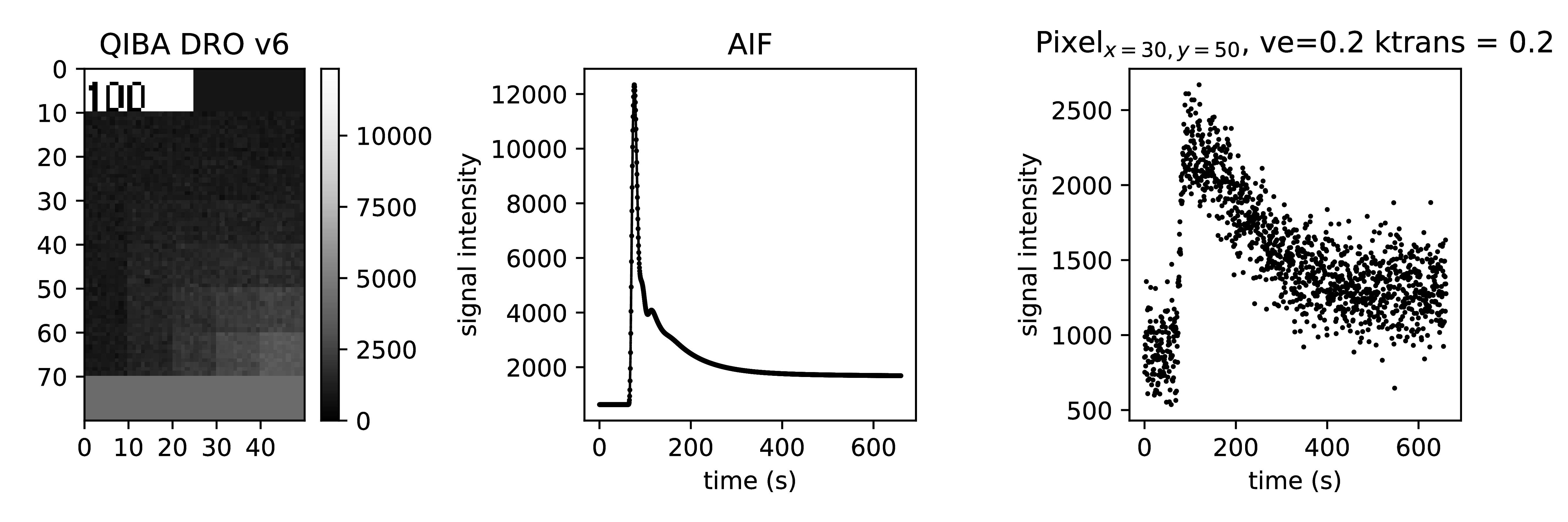
Validation To validate the parameter estimates of the BTM, the QIBA_v6_Tofts1 DRO, provided by the Quantitative Imaging Biomarkers Alliance (QIBA), was used. The DRO contains tissue concentration curves constructed with the standard Toft’s model (TM)2 for an arterial input function (AIF) and 30 combinations of $$$K^{trans}$$$ and $$$v_e$$$ (Fig. 1). For a more realistic setting, complex Gaussian noise with standard deviation $$$\sigma$$$=0.2 relative to the baseline signal was added. The concentration-time curves were fitted with the NLLS approach using the L-BFGS-B3 algorithm via python’s scipy4 package. A bootstrapping5 method was applied to assess the uncertainty in parameter estimation.
A BTM was implemented in stan6 which infers the parameter’s posterior distribution via Bayes’ theorem $$P(\theta\mid D)={\frac {P(D\mid \theta)\,P(\theta)}{P(D)}}$$ and Markov Chain Monte Carlo (MCMC) methods using the NUTS7 algorithm. For both methods, the percentage error was calculated between estimated parameters and ground truth. Uncertainty $$$\sigma$$$ was inferred from half the width (17th-83rd percentile) of bootstrap samples and posterior distributions. The structural similarity index (SSIM)8 was calculated between estimated and true maps, and between both uncertainty maps to quantify differences.
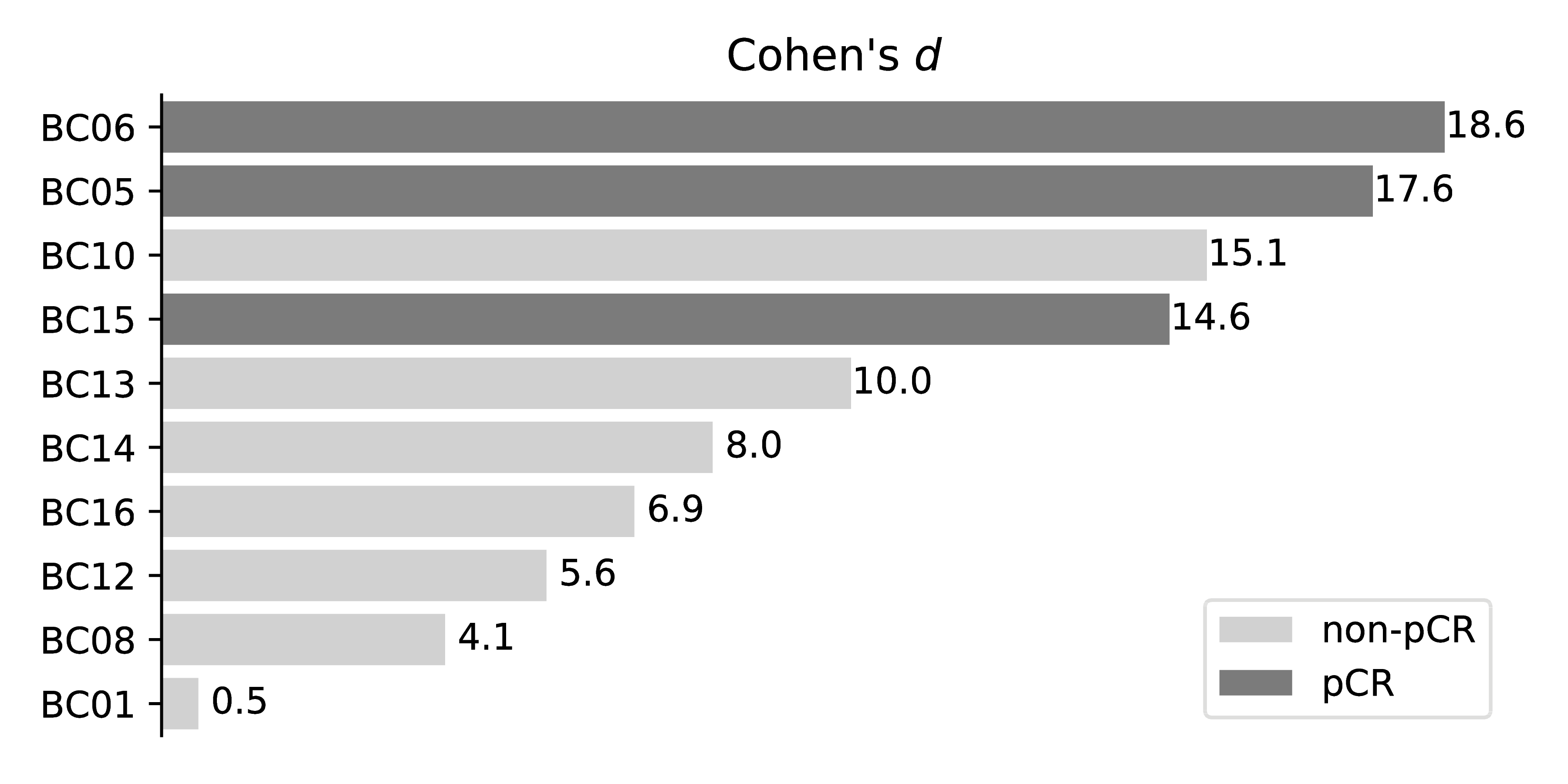
Application A set of breast DCE-MRI data9 was used, acquired from 10 patients before and during preoperative neoadjuvant chemotherapy (NACT), provided by the Quantitative Imaging Network (QIN). Patients were labeled according to their pathologic response – 3 pathologic complete responder (pCR) and 7 non-pCR. Concentration curves averaged within regions of interest (ROI) were evaluated with the BTM. Posterior distributions for $$$K^{trans}$$$ were compared between visits and the change was assessed by means of Cohen’s d, calculated as: $$d={\frac {{\bar{x}}_{1}-{\bar{x}}_{2}}{{\sqrt{(\sigma_{1}^{2}+\sigma_{2}^{2})/2}}}}.$$ A univariate logistic regression (ULR) model was fit to the Cohen’s d values to obtain a prediction of response to NACT.
Results
Fig. 2 shows the fitted median-$$$K^{trans}$$$ values of the DRO for the BTM (SSIM 95%) and point estimates for NLLS (SSIM 91%) on the left. The middle column displays the calculated percentage error. The uncertainty maps from posterior distributions and bootstrap samples are shown on the right, coinciding with a SSIM of 91%. Regions for $$$v_e$$$=0.01 are difficult to infer for both methods, indicated by the highest percentage error and uncertainty.
Fig. 3 shows the posterior distributions for $$$K^{trans}$$$ for visit 1 (blue) and visit 2 (orange) for all patients. Cohen’s d values are visualized in Fig. 4; light-gray represents non-pCR, dark-gray pCR. The ULR analysis revealed an area under the receiver operator curve (AUC) of 0.952.
Discussion
In this study, we assessed posterior probability distributions of tracer-kinetic parameters obtained with a BTM against a standard NLLS approach. Validation with a DRO revealed high accuracy of BTM and NLLS approaches, indicated by strong similarity between estimated and ground truth maps. In addition, precision of estimates, assessed via the width of the posterior probability distributions and bootstrapping, respectively, was in very good agreement between both approaches.
The breast cancer DCE-MRI dataset revealed that the degree of decrease in $$$K^{trans}$$$ gives information about the pathologic response to NACT. The response, including measures of uncertainty of the parameter estimates, was quantified with Cohen’s d, calculated from the posterior distributions between visit 1 and 2. ULR modeling indicated excellent prediction of response. Further analysis could include a model selection step to decrease the influence of systematic modeling errors on posterior distributions and may further improve assessment of therapy response.
Conclusion
We evaluated a BTM with a DRO, assessed accuracy and precision against the standard NLLS approach and showed how posterior distributions are used to assess therapy response. In conclusion, we demonstrated that Bayesian modeling provides an elegant means to assess posterior probability distributions, which are in good agreement with established approaches.Acknowledgements
This work was supported by the research training group GRK 2274 of the DFG, Deutsche Forschungsgemeinschaft.References
1. Daniel P. Barboriak Lab (2014). QIBA Content. https://sites.duke.edu/dblab/qibacontent/. Accessed February 1, 2018.
2. Tofts, P. S. and Kermode, A. G. (1991). Measurement of the blood-brain barrier permeability and leakage space using dynamic MR imaging. 1. Fundamental concepts. Magnetic Resonance in Medicine, 17(2):357–367.
3. Zhu, C., Byrd, R. H., Lu, P., and Nocedal, J. (1997). Algorithm 778: L-BFGS-B: Fortran Subroutines for Large-scale Bound-constrained Optimization. ACM Trans. Math. Softw., 23(4):550–560.
4. Jones, E., Oliphant, T., and Peterson, P. (2001). SciPy: Open source scientific tools for Python.
5. Kershaw, L. E. and Buckley, D. L. (2006). Precision in measurements of perfusion and microvascular permeability with T1-weighted dynamic contrast-enhanced MRI. Magnetic Resonance in Medicine, 56(5):986–992.
6. Carpenter, B., Gelman, A., Hoffman, M. D., Lee, D., Goodrich, B., Betancourt, M., Brubaker, M., Guo, J., Li, P., and Riddell, A. (2017). Stan : A Probabilistic Programming Language. Journal of Statistical Software, 76(1).
7. Homan, M. D. and Gelman, A. (2014). The No-U-turn Sampler: Adaptively Setting Path Lengths in Hamiltonian Monte Carlo. J. Mach. Learn. Res., 15(1):1593–1623.
8. Wang, Z., Bovik, A., Sheikh, H., and Simoncelli, E. (2004). Image Quality Assessment: From Error Visibility to Structural Similarity. IEEE Transactions on Image Processing, 13(4):600–612.
9. Huang, Wei, Tudorica, Alina, Chui, Stephen, Kemmer, Kathleen, Naik, Arpana, Troxell, Megan, Holtorf, Megan. (2014). Variations of dynamic contrast-enhanced magnetic resonance imaging in evaluation of breast cancer therapy response: a multicenter data analysis challenge. The Cancer Imaging Archive. http://doi.org/10.7937/K9/TCIA.2014.A2N1IXOX
Figures