0695
Estimation of low frequency conductivity from Larmor frequency conductivity1Philips Research, Hamburg, Germany
Synopsis
EEG source localization requires the conductivity map of the patient's head. Patient-individual conductivity maps can be measured in the framework of MRI using "Electric Properties Tomography" (EPT). However, EEG source localization requires the conductivity belonging to low frequency (LF) range instead radiofrequency (RF) range, as it is the case for EPT. To solve this problem, this study suggests two EPT measurements at different B0, and to transform the resulting conductivities from RF to LF via a simplified Cole-Cole-model. The approach has been validated with organic and non-organic phantoms as well as with volunteer brain experiments.
Introduction
Electroencephalography (EEG) source localization requires the conductivity map of patients’ head, and accuracy of this source localization benefits from patient-individual conductivity maps. Such maps can be measured with MRI using "Electric Properties Tomography" (EPT, [1]). However, EEG source localization requires conductivity for low frequency range (LF, ~100-1000 Hz) instead radiofrequency range (RF, ~50-500 MHz), as obtained from EPT. To solve this problem, it was suggested to transform conductivity from RF to LF via the relationship between extra/intracellular space, estimated by several model assumptions based on diffusion weighted imaging [2]. As an alternative, this study suggests multiple EPT measurements at different main fields B0, thus different Larmor frequencies in the RF range, and to transform resulting conductivities from RF to LF via a simplified Cole-Cole model (sCCM) based on the full Cole-Cole-model (fCCM) described in [3].Theory
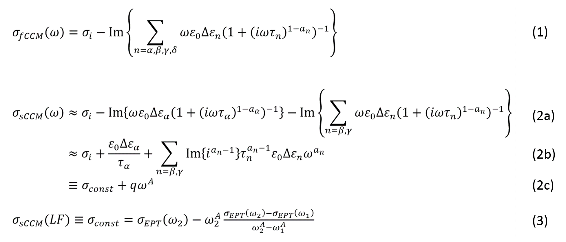
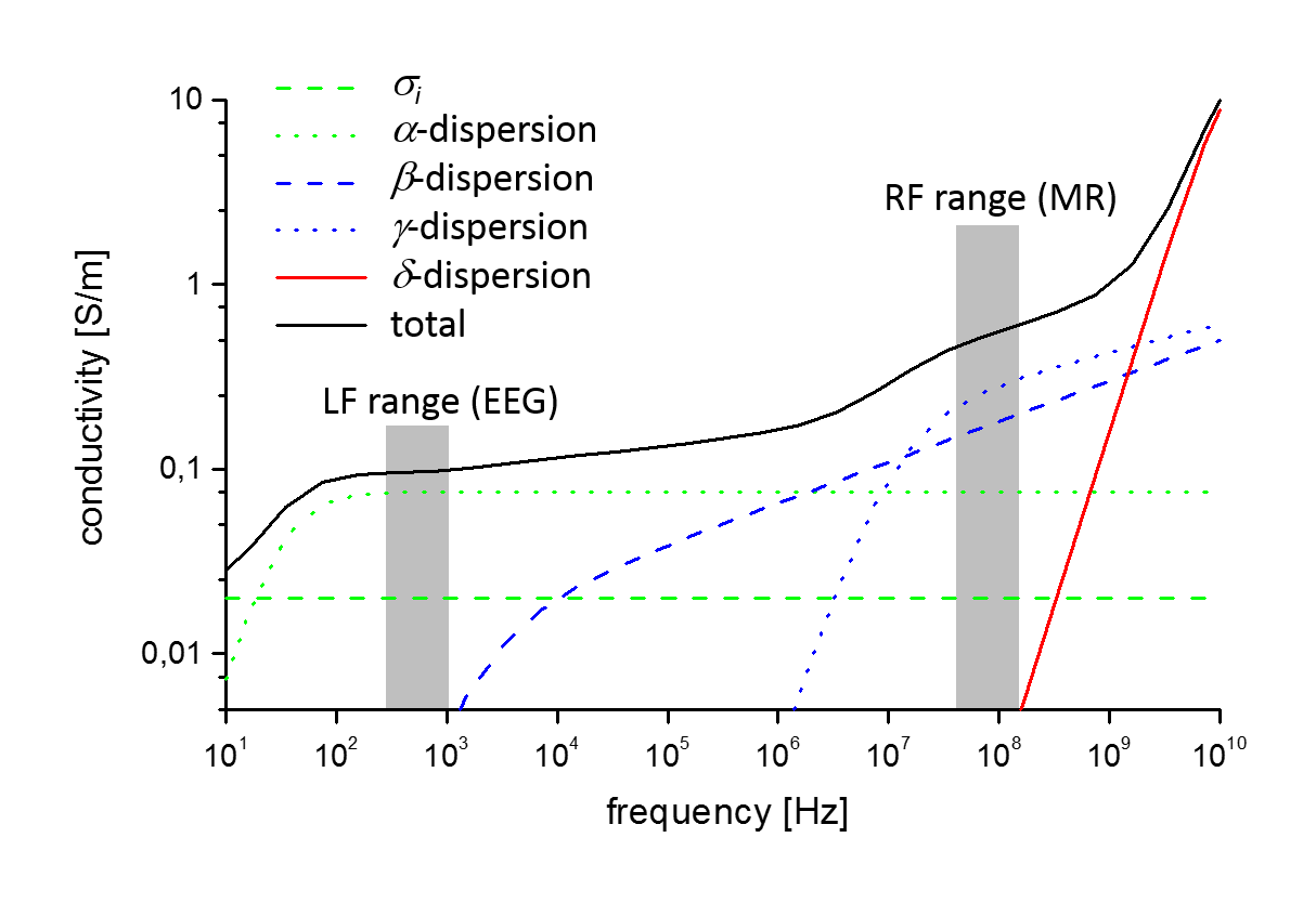
Conductivity depends on frequency ω as described by the fCCM [3], including α/β/γ/δ-dispersion observed at different frequencies, and an ionic conductivity σi independent of ω (Eq.(1) in Fig.1). In the RF range, typical tissue conductivity spectra (shown in Fig.2 exemplarily for grey matter) can be approximated by a constant term (reflecting σi and α-dispersion) and an exponential term (reflecting β/γ-dispersion) (Eq.(2) in Fig.1). The resulting sCCM separates these two terms by measuring conductivity at two different RF values (Eq.(3) in Fig.1). The unknown LF conductivity can be approximated by the constant term of the RF spectrum (Fig.2). Since δ-dispersion becomes relevant only above RF range, it was neglected in this study. According to [3], cerebrospinal fluid (CSF) is the only head tissue type inappropriate for sCCM, and thus the more suitable approximation σ(1kHz) ~ σ(64MHz) was applied for CSF.Methods
The approach was validated via (A) brain literature data, (B) phantoms experiments, (C) brain volunteer experiments.
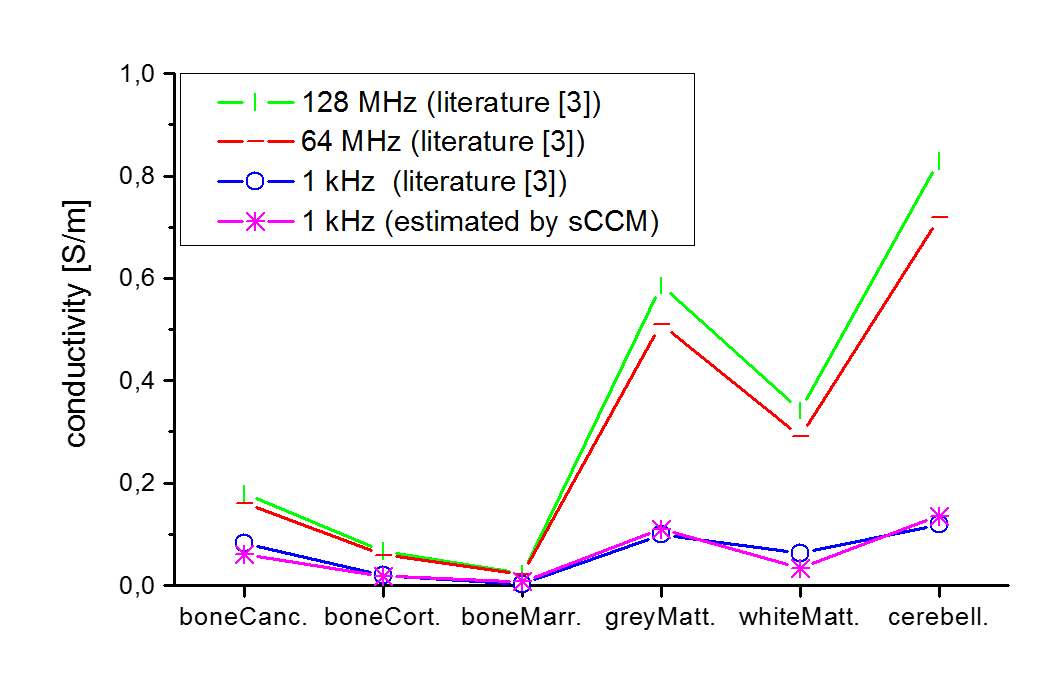
(A) Brain literature data: For 6 head tissue types, Eq.(3) was applied to estimate ssCCM(1kHz) from σfCCM(128MHz) and σfCCM(64MHz) taken from [3], and compared with σfCCM(1kHz) from [3].
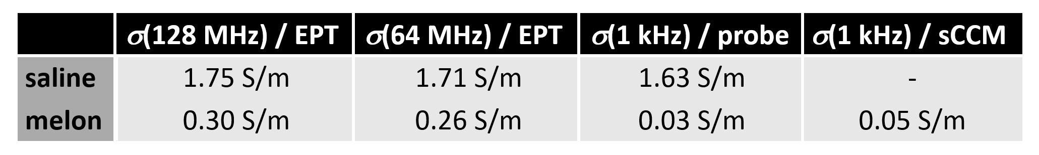
(B) Phantom experiments: A water melon (representing white matter) and a saline phantom (11g NaCl / liter H2O, representing CSF) have been measured at 1.5T and 3T (Ingenia, Philips, Netherlands) with a DREAM sequence [4] (voxel 4x4x8 mm3, imaging angle 10°, STEAM angle 50°, TR/TE1/TE2(1.5T)=8.8/2.7/4.6ms, TR/TE1/TE2(3T)=4.4/1.6/2.3ms) and a steady state free precession (SSFP) sequence (voxel 1x1x1 mm3, flip angle 30°, TR/TE(1.5 T)=3.8/1.9ms, TR/TE(3T)=3.5/1.7ms). EPT reconstruction was performed as in [5] with B1 magnitude from DREAM and phase from SSFP yielding σ(128MHz) and σ(64MHz). Subsequently, the mean of σ(128MHz) and σ(64MHz) averaged over 3x3x3cm3 of melon’s center entered Eq.(3) to estimate σsCCM(1kHz). An impedance analyzer (4294A, Agilent, USA) was used to independently measure σ(1kHz) of saline and melon.
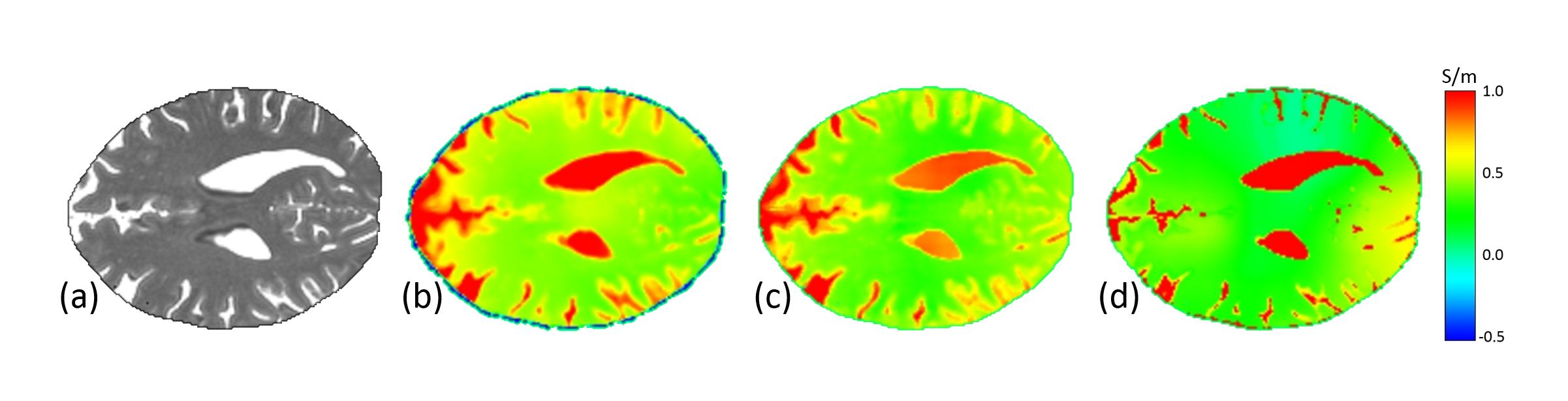
(C) Brain volunteer experiments: After obtaining informed written consent according to local Institutional Review Board, the brains of 4 healthy volunteers (mean age 42±6 yrs) were measured in analogy to phantom experiments (B). After EPT reconstruction, conductivity maps of B0=3T were registered onto conductivity maps of B0=1.5T, and Eq.(3) was applied voxel by voxel. The result was median filter as in [5]. CSF pulsation artefacts were compensated by taking upper quartile of CSF conductivity [6] after identifying CSF voxels by signal thresholding of SSFP magnitude. The corresponding value of σ(64MHz) was assigned to σ(1kHz) as explained above.
Results
(A) Averaged over all tissue types regarded, the difference between literature σfCCM(1kHz) [3] and estimated σsCCM(1kHz) is σerr=0.014S/m (Fig.3).
(B) Phantom results are summarized in Fig.4.
(C) Brain results are shown for one of the volunteers in Fig.5. Similar results were obtained for the other volunteers.
Discussion and Outlook
The study showed that a simplified Cole-Cole model (sCCM) is able to estimate LF conductivity from RF conductivity. While the theoretical part of the study suggests that sCCM is applicable for a wide range of tissue types, the in-vivo validation was essentially restricted to gray and white matter. CSF was also taken into account, but needed special treatment not only due to its particular frequency behaviour (not covered by sCCM), but also due to pulsation artefacts arising from the lack of cardiac triggering of the in-vivo scans performed [6]. Bone and bone marrow theoretically fulfil sCCM, but for in-vivo validation, dedicated sequences [7] shall be applied in a follow-up study. Without specific parameter adaptation, sCCM has proven to be applicable to the majority of head tissue types, thus potentially also applicable to pathologic tissue types, where no conductivity spectra are available.
Follow-up studies shall also address further extensions of the sCCM, like extending the range of B0 from the applied 1.5-3T to e.g. 0.5-7T, or additionally taking permittivity into account.
Acknowledgements
The authors would like thank Kay Nehrke for supporting DREAM B1 mapping and Lyubomir Zagorchev and Sergei Turovets for supporting discussions.References
[1] Katscher U et al., Electric properties tomography: Biochemical, physical and technical background, evaluation and clinical applications. NMR Biomed. 2017;30:3729
[2] Sajib SZ et al., Electrodeless conductivity tensor imaging (CTI) using MRI: basic theory and animal experiments. Biomed Engin Lett. 2018;8:273
[3] Gabriel S et al., The dielectric properties of biological tissues: III. Parametric models for the dielectric spectrum of tissues. Phys Med Biol. 1996;41:2271
[4] Nehrke K et al., DREAM - a novel approach for robust, ultrafast, multislice B1 mapping. Magn Reson Med. 2012;68:1517
[5] Tha KK et al., Noninvasive electrical conductivity measurement by MRI: a test of its validity and the electrical conductivity characteristics of glioma. Eur Radiol. 2018;28:348
[6] Katscher U et al., The impact of CSF pulsation on reconstructed brain conductivity. Proc. ISMRM 2018;26:546
[7] Lee SK et al., Tissue electrical property mapping from zero echo-time magnetic resonance imaging. IEEE Trans Med Imag. 2015;34:541
Figures