Flow & Velocity Imaging

Martin Graves¹

¹Cambridge Univ. Hosp. NHS Found. Trust, United Kingdom

Synopsis

The standard method of quantifying cardiovascular velocity and flow in MRI is to use a phase contrast (PC) imaging technique. This presentation will describe the basic principles of the PC method, its practical implementation and clinical optimisation.

Target Audience

MR scientist/engineers and clinicians interested in the quantification of blood velocity and flow.

Outcome/Objectives

Understand the principles of phase contrast techniques and how to apply the methods in research and clinical practice.

Principles

The effects of motion on the NMR signal was well known before the development of MRI. Both magnitude effects, due to spin washout, and phase effects due to motion along a magnetic field gradient were described in the 1950s/60s. A review of the early work around velocity and flow effects in MRI was published by Axel in 1984 (1).

Moran in 1982 (2) introduced the concept of encoding the velocity of a spin into the complex NMR signal, a technique that he called a ‘flow-velocity zeugmatographic interlace’. Several groups then developed this technique into a method to directly encode velocity into the phase of the signal using balanced gradient pulses (3-5). It was, however, noted that the background field uniformity was a confounder to the accuracy of the technique, particularly for gradient echo based sequences. To eliminate these background phase shifts two acquisitions are performed along each gradient direction with the bipolar velocity-encoding gradients modified for the second acquisition. The phase images for both acquisitions are then calculated and subtracted, cancelling the stationary background phase and leaving only positive and negative phase shifts depending upon the direction of blood flow (6). Spins moving with a velocity $$$v$$$ along the direction of a magnetic field gradient of amplitude $$$G$$$ and duration $$$T$$$ accumulate phase according to $$$\phi=\gamma\cdot v\cdot G\cdot T^2$$$. The product $$$ G\cdot T^2$$$ is usually referred to as the first moment of the gradient $$$(M_1)$$$. If we perform two acquisitions with different first moments, then the phase difference is given by $$$\triangle\phi=\gamma\cdot v\cdot \triangle M_1$$$.

The phase/velocity relationship is scaled through a user-controlled velocity encoding value, known as the venc. Since we have $$$2\pi$$$ of unique phase available, flow in one direction, relative to the gradient direction, is allocated $$$0$$$ to $$$+\pi$$$, whilst flow in the opposite direction is allocated $$$0$$$ to $$$-\pi$$$. The venc is the maximum velocity, along each direction, that will result in a $$$\pi$$$ phase shift, i.e. $$$ venc=\frac{\pi}{\gamma\cdot\triangle M_1}$$$.

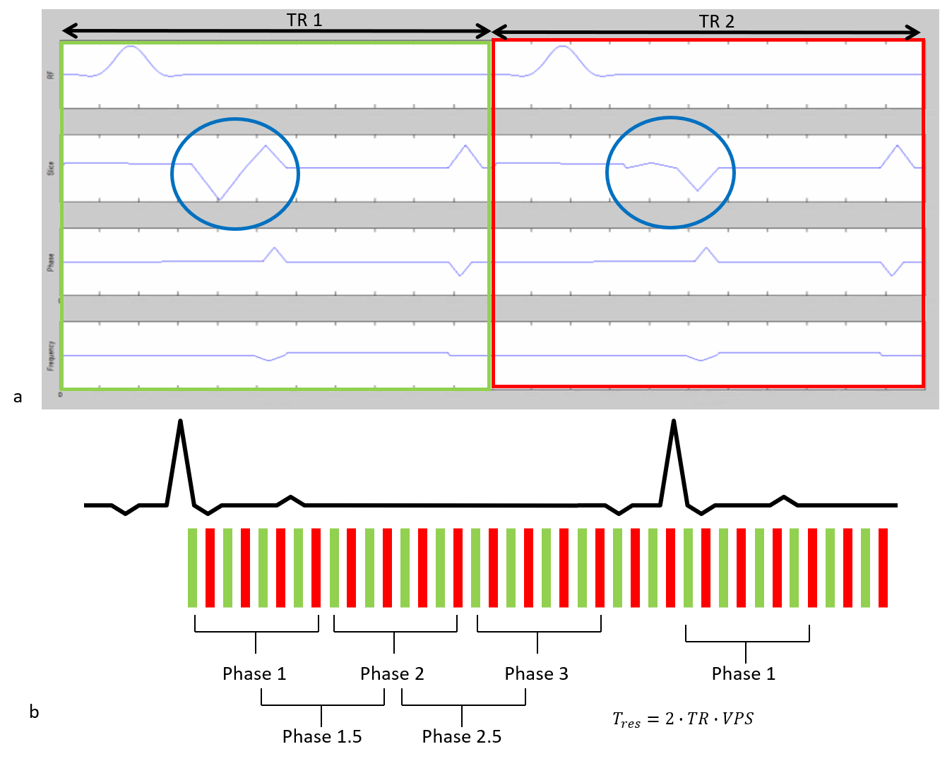
To minimise the echo time (TE) the velocity encoding gradients are usually combined with the imaging gradients. In a ‘asymmetric’ acquisition, one acquisition has the gradients calculated to yield a zero-phase shift for spins moving with a constant velocity, i.e.,$$$M_1=0$$$. In the second acquisition the gradient amplitudes are modified to yield the desired phase/velocity sensitivity. In a ‘symmetric’ acquisition the phase/velocity sensitivity is shared equally between the two acquisitions $$$(\pm \frac{\triangle M_1}{2})$$$ (7). Figure 1(a) shows two adjacent TR periods for a ‘symmetric’ acquisition.

Acquisition

In quantitative velocity/flow imaging we usually perform a single slice PC acquisition perpendicular to the direction of the vessel, i.e. through plane encoding. Usually a multiple temporal-phase acquisition is performed that is synchronised to the subjects’ cardiac cycle. Such an acquisition is often termed cine phase contrast (CPC) imaging. The velocity-encoding gradients are usually applied along the slice selection direction to quantify velocities through the slice, and the two encodings are usually interleaved within the same heartbeat to minimize spatial misregistration. Fast imaging methods such as segmented k-space acquisitions (8) are often used with CPC imaging, as they are in standard functional cardiac imaging, to reduce overall acquisition times Figure 1(b) shows a segmented PC acquisition. 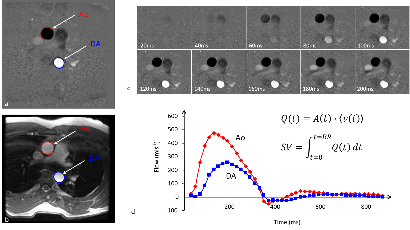However, care needs to be taken in terms of the effective temporal resolution of the acquisition since increasing the segment duration results in an increased smoothing or low-pass filtering of the time-resolved flow waveform (9). Figure 2 shows images from a typical CPC acquisition.

Analysis

Analysis of the images generally involves outlining of the vessel on the magnitude images and applying the outline to the phase image. The average phase value within the region can then be converted into an average velocity (ms^-1). Furthermore, since we know the area (m²) of the region for each temporal phase we can multiply that by the mean velocity to obtain the instantaneous flow volume (m³s^-1). In addition to average velocities it is possible to determine the peak velocity within the region as this may also be diagnostically useful. If the actual velocity exceeds the user-selected venc then aliasing will occur. It is possible to ‘unwrap’ this aliasing otherwise it will be necessary to repeat the acquisition using a higher venc. Note that velocity images will appear noisier as the venc is increased. Providing that the velocity $$$v < venc$$$ then the signal-to-noise ratio (SNR) of the phase difference image can be expressed as $$$SNR_{\triangle\phi}\propto SNR_M\cdot\frac{v}{venc}$$$ , where $$$ SNR_M$$$ is the SNR of the magnitude image (10).

Errors

Even though the phase images from positive and negative flow encodings are subtracted to eliminate background phase errors, there may be residual errors due to the different eddy currents produced by the different flow encoding gradient amplitudes. These errors appear as offsets in the data, so typically the stationary background is no longer zero. Some correction of the background signal offset may therefore be required, otherwise regurgitant or shunt flow measurement accuracy may be compromised (11). Other residual phase errors such as those due to concomitant fields/Maxwell terms (12) and gradient field non-linearities (13) can also be corrected. The accuracy of CPC measurements can also be affected by several imaging parameters, such as ensuring there are at least 16 pixels covering the vessel area and using high receiver bandwidths and an in-phase TE to minimise the effects of chemical shift-induced phase errors (10, 14).

4D Methods

Velocity mapping can also be performed in-plane by applying the flow-encoding gradients on the appropriate axis. Furthermore, it is possible to acquire velocity data along all three directions, which when combined as part of multi temporal phase 3D acquisition can provide 4D velocity quantification and visualisation. This data can be used to measure velocity/flow in any orientation and also used to calculate temporally-resolved 4D flow vectors and streamlines. These acquisitions are quite time consuming and require either respiratory gating, typically using navigators, or signal averaging (15).

Acknowledgements

No acknowledgement found.

References

1. Axel L. Blood flow effects in magnetic resonance imaging. AJR Am J Roentgenol. 1984; 143(6): 1157-66.

2. Moran PR. A flow velocity zeugmatographic interlace for NMR imaging in humans. Magn Reson Imaging. 1982; 1(4): 197-203.

3. Bryant DJ, Payne JA, Firmin DN, Longmore DB. Measurement of flow with NMR imaging using a gradient pulse and phase difference technique. J Comput Assist Tomogr. 1984; 8(4): 588-93.

4. van Dijk P. Direct cardiac NMR imaging of heart wall and blood flow velocity. J Comput Assist Tomogr. 1984; 8(3): 429-36.

5. Wedeen VJ, Rosen BR, Chesler D, Brady TJ. MR velocity imaging by phase display. J Comput Assist Tomogr. 1985; 9(3): 530-6.

6. Ridgway JP, Smith MA. A technique for velocity imaging using magnetic resonance imaging. Br J Radiol. 1986; 59(702): 603-7.

7. Bernstein MA, Shimakawa A, Pelc NJ. Minimizing TE in moment-nulled or flow-encoded two- and three-dimensional gradient-echo imaging. J Magn Reson Imaging. 1992; 2(5): 583-8.

8. Foo TK, Bernstein MA, Aisen AM, Hernandez RJ, Collick BD, Bernstein T. Improved ejection fraction and flow velocity estimates with use of view sharing and uniform repetition time excitation with fast cardiac techniques. Radiology. 1995; 195(2): 471-8.

9. Polzin JA, Frayne R, Grist TM, Mistretta CA. Frequency response of multi-phase segmented k-space phase-contrast. Magn Reson Med. 1996; 35(5): 755-62.

10. Nayak KS, Nielsen JF, Bernstein MA, Markl M, P DG, R MB, et al. Cardiovascular magnetic resonance phase contrast imaging. J Cardiovasc Magn Reson. 2015; 17: 71.

11. Gatehouse PD, Rolf MP, Graves MJ, Hofman MB, Totman J, Werner B, et al. Flow measurement by cardiovascular magnetic resonance: a multi-centre multi-vendor study of background phase offset errors that can compromise the accuracy of derived regurgitant or shunt flow measurements. J Cardiovasc Magn Reson. 2010; 12: 5.

12. Bernstein MA, Zhou XJ, Polzin JA, King KF, Ganin A, Pelc NJ, et al. Concomitant gradient terms in phase contrast MR: analysis and correction. Magn Reson Med. 1998; 39(2): 300-8.

13. Markl M, Bammer R, Alley MT, Elkins CJ, Draney MT, Barnett A, et al. Generalized reconstruction of phase contrast MRI: analysis and correction of the effect of gradient field distortions. Magn Reson Med. 2003; 50(4): 791-801.

14. Lotz J, Meier C, Leppert A, Galanski M. Cardiovascular flow measurement with phase-contrast MR imaging: basic facts and implementation. Radiographics. 2002; 22(3): 651-71.

15. Markl M, Chan FP, Alley MT, Wedding KL, Draney MT, Elkins CJ, et al. Time-resolved three-dimensional phase-contrast MRI. J Magn Reson Imaging. 2003; 17(4): 499-506.

Figures

a) shows two TRs of a PC sequence incorporating additional bipolar gradients (ringed in blue) to encode velocity into the signal phase. The two encodings (green and red) are performed in subsequent TRs. In this example the encodings are applied along the slice select direction to encode velocity through the slice. In (b) the encodings are shown as part of a retrospectively gated segmented k-space acquisition. Multiple views are acquired in each R-R interval. In this case four views are acquired for each encoding. Since the temporal resolution is 8xTR in this example, view sharing has been used to improve the apparent temporal resolution.

Images from a typical CPC acquisition through the ascending aorta (Ao) and descending aorta (DA). (a) shows the phase/velocity image and (b) shows the magnitude image from a single temporal phase. (c) Shows the first ten temporal phases. (d) Shows the flow-time curve. The flow (ml s^-1) at each temporal phase is obtained by multiplying the average velocity in each ROI (mm s^-1) with the area (mm²). If the instantaneous flow is plotted against time for all the temporal phases, the area under the curve represents the stroke volume (SV). Multiplying the SV by the heart rate gives the cardiac output (ml min^-1).

Proc. Intl. Soc. Mag. Reson. Med. 26 (2018)