Synopsis

We will discuss the Human Connectome Project’s multi-modal cortical parcellation version 1.0—the data acquisition and analysis requirements, how the parcellation was made, and how it can be applied to individuals. This state of the art map of the cerebral cortex was made possible by using exceptionally high quality MRI data precisely aligned across individuals. Cortical areal boundaries were identified when visible in multiple modalities and areas were painstakingly related to the neuroanatomical literature. A machine learning classifier was then trained to automatically identify each cortical area based on its multi-modal fingerprint in individual subjects, replicating the parcellation.

For over a century making a map of the human cerebral cortex has been an objective of neuroscience. Understanding the specialized information processing units of cortex, the cortical areas, requires that they be delineated in an accurate and reproducible way. Historically, cortical areas have been defined based on microstructural architecture, functional properties, area-to-area connectivity, or within-area mesoscale organization—topography (Van Essen and Glasser 2018). Many of these studies were carried out using invasive techniques in post-mortem human tissues or in non-human primates. Here we capitalized on the high quality Human Connectome Project (HCP) MRI data that allows us to measure architecture (cortical thickness and T1-weighted/T2-weighted myelin maps), function (task-based functional MRI), connectivity (resting state functional MRI connectivity), and topography (resting state functional MRI visuotopic connectivity) non-invasively in living human subjects (Glasser et al 2016a).

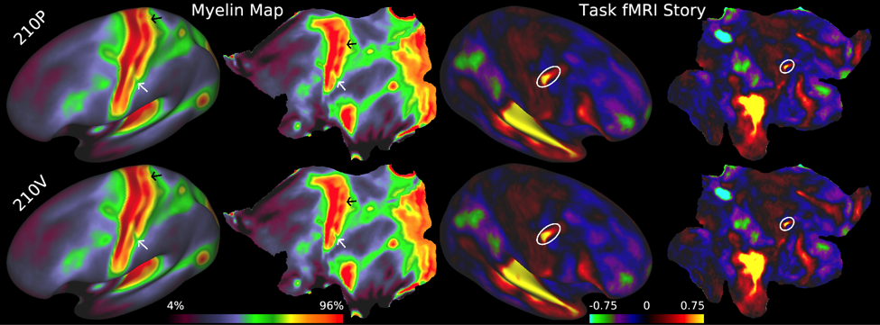
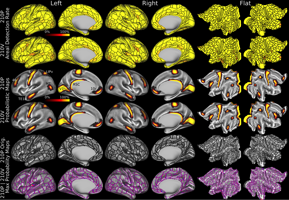
Accurately mapping human cortical areas required rethinking how brain imaging data are acquired, analyzed, and shared (Glasser et al 2016b). We acquired structural and functional MRI data at much higher spatial and temporal resolution than is traditionally done, including T1-weighted and T2-weighted images at 0.7mm isotropic, fMRI at 2mm isotropic with a repetition time of 720ms (requiring a multi-band EPI acquisition; Feinberg et al 2010), together with matched fieldmap images to correct the distortions between different MRI image types. Unlike in traditional neuroimaging, we minimized overt spatial smoothing (and interpolation-related smoothing) and aligned cortical data across subjects on the surface (to a combined set of cortical surface vertices and subcortical voxels known as ‘grayordinates’ that are stored in the CIFTI file format; Glasser et al 2013). Our surface-based registration was driven by the same features that define cortical areas, such as myelin maps, resting state networks maps, and resting state visuotopic maps, rather than cortical folding patterns (Robinson et al 2014; 2018). This improvement resulted in substantially sharper group average maps that were highly reproducible across two independent groups of 210 subjects (210P and 210V, Figure 1).

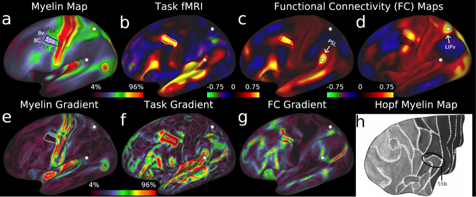
To map cortical areas, we used locations of sharp change in group average myelin maps, cortical thickness maps, task-based functional activation maps, and functional connectivity maps from the 210P group. We focused on locations where these gradients co-localized across more than one modality to take advantage of converging and complementary evidence (Figure 2). We also mapped some areas with visuotopic resting state functional connectivity. We used a semi-automated parcellation approach, where neuroanatomists chose the maps most useful for each areal boundary and drew an initial guess at its location and then used an algorithm to draw the final boundary that best fit the available data. This semi-automated approach allowed for quality control of each areal boundary to avoid artifactual boundaries. Importantly, each boundary also underwent statistical testing to show that there was a strong and statistically significant difference across the boundary in more than one measure. The last step involved painstaking description of each cortical area and relating it to the neuroanatomical literature to see if the area had previously been described.

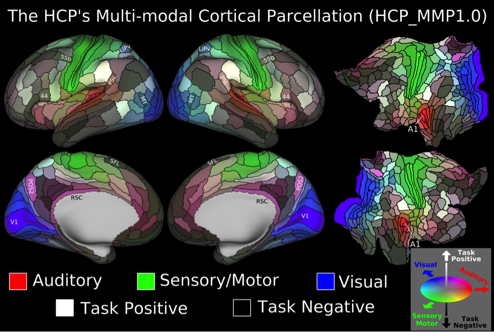
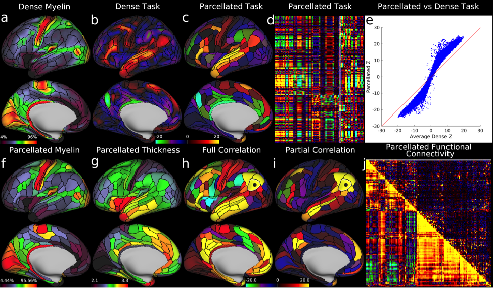
We found 180 cortical areas in each hemisphere, 83 of which had previously been described and 97 new areas (Figure 3). These areas showed striking bilateral symmetry that matched the input data (Figure 1) in both their boundaries and their association with the three main sensory input streams of the brain: auditory (red), somatosensory (green), and visual (blue), and two anti-correlated cognitive systems, the task negative or default mode (dark) and the task-positive or anti-default mode (bright). Importantly these cortical areas were strongly and statistically significantly different across the areal boundaries even in the independent dataset (210V). These cortical areas can be used in ‘parcellated analyses’ where neuroimaging measures such as myelin content, cortical thickness, and task-based or resting state functional activity timeseries are averaged to improve SNR in a neuroanatomically sensible form of spatial smoothing (Figure 4).

This map took years to complete using the semi-automated neuroanatomist driven approach, which would be impractical for application to individual subjects. For this reason, we trained a machine learning classifier (Hacker et al 2013) to recognize the unique multi-modal fingerprint of each cortical area. This classifier was able to identify these areas in individual subjects automatically, even in cases where areas had atypical relationships with their neighbors relative to the group pattern. Indeed the areal classifier detected 96.6% of cortical areas in the 210V dataset that was not used for either parcellation or classifier training and reproduced the parcellation at the group level with a correlation of r=0.965 (Figure 5)—very similar to that of the starting data (Figure 1).

To best make use of this new map of the brain and areal classifier, one needs only to acquire high resolution T1-weighted and T2-weighted structural MRI (0.8mm isotropic or better), resting state fMRI (2.4mm or better with 1s repetition time or better), and a field map, as leaving out the HCP’s specialized task fMRI battery resulted in an areal detection rate of 96.4%—essentially the same as with it included. These same images will allow the investigator to preprocess their data with the HCP Pipelines, align their data with the areal-feature-based ‘MSMAll’ surface-based registration software, and run the areal classifier. Additionally the investigator will be able to use the HCP’s functional MRI denoising software including spatial ICA + the FIX component classifier (Salimi-Khorshidi et al 2014) and the new temporal ICA-based selective global noise cleanup approach that avoids the need to choose between using or not using global signal regression (Glasser et al 2018). Because this map is the product of an improved, HCP-Style, approach to brain imaging, it is difficult to relate it accurately to traditional brain imaging studies (Coalson et al 2018). Fortunately tools are being developed to aid investigators in bringing legacy data to the HCP’s multi-modal map by allowing such data to be reprocessed in a way compatible with modern surface-based cortical parcellations (Dickie et al 2018). We anticipate that this new map and the improved approach to brain imaging it was derived from will accelerate progress in understanding the brain in health and disease.

Acknowledgements

References

Coalson, T.S., Van Essen, D.C., Glasser, M.F. Preprint. Lost in Space: The Impact of Traditional Neuroimaging Methods on the Spatial Localization of Cortical Areas. bioRxiv 255620; doi: https://doi.org/10.1101/255620.

Dickie, E.W. Anticevic, A. Smith, D.E. Coalson, T.S. Manogaran, M., Viviano, J.D. Glasser, M.F., Van Essen, D.C., Voineskos, A.N. Software and Manuscript In Preparation. ciftify: A framework for surface-based analysis of legacy MR acquisitions. https://github.com/edickie/ciftify.

Feinberg, D.A., Moeller, S., Smith, S.M., Auerbach, E., Ramanna, S., Glasser, M.F., Miller, K.L., Ugurbil, K. and Yacoub, E., 2010. Multiplexed echo planar imaging for sub-second whole brain FMRI and fast diffusion imaging. PloS one, 5(12), p.e15710.

Glasser, M.F., Sotiropoulos, S.N., Wilson, J.A., Coalson, T.S., Fischl, B., Andersson, J.L., Xu, J., Jbabdi, S., Webster, M., Polimeni, J.R. Van Essen, D.C., and Jenkinson, M., 2013. The minimal preprocessing pipelines for the Human Connectome Project. Neuroimage, 80, pp.105-124.

Glasser, M.F., Coalson, T.S., Robinson, E.C., Hacker, C.D., Harwell, J., Yacoub, E., Ugurbil, K., Andersson, J., Beckmann, C.F., Jenkinson, M. Smith, S.M., and Van Essen, D.C. 2016a. A multi-modal parcellation of human cerebral cortex. Nature, 536(7615), pp.171-178.

Glasser, M.F., Smith, S.M., Marcus, D.S., Andersson, J.L., Auerbach, E.J., Behrens, T.E., Coalson, T.S., Harms, M.P., Jenkinson, M., Moeller, S. Robinson, E.C., Sotiropoulos, S.N., Xu, J., Yacoub, E., Ugurbil, K., and Van Essen, D.C. 2016b. The human connectome project's neuroimaging approach. Nature Neuroscience, 19(9), p.1175.

Glasser, M.F., Coalson, T.S., Bijsterbosch, J.D., Harrison, S.H., Harms, M.P., Anticevic, A., Van Essen, D.C., Smith, S.M. Preprint. Using Temporal ICA to Selectively Remove Global Noise While Preserving Global Signal in Functional MRI Data. bioRxiv 193862; doi: https://doi.org/10.1101/193862.

Hacker, C.D., Laumann, T.O., Szrama, N.P., Baldassarre, A., Snyder, A.Z., Leuthardt, E.C. and Corbetta, M., 2013. Resting state network estimation in individual subjects. Neuroimage, 82, pp.616-633.

Robinson, E.C., Jbabdi, S., Glasser, M.F., Andersson, J., Burgess, G.C., Harms, M.P., Smith, S.M., Van Essen, D.C. and Jenkinson, M., 2014. MSM: a new flexible framework for Multimodal Surface Matching. Neuroimage, 100, pp.414-426.

Robinson, E.C., Garcia, K., Glasser, M.F., Chen, Z., Coalson, T.S., Makropoulos, A., Bozek, J., Wright, R., Schuh, A., Webster, M. Hutter, J., et al. 2018. Multimodal surface matching with higher-order smoothness constraints. NeuroImage, 167, pp.453-465.

Salimi-Khorshidi, G., Douaud, G., Beckmann, C.F., Glasser, M.F., Griffanti, L. and Smith, S.M., 2014. Automatic denoising of functional MRI data: combining independent component analysis and hierarchical fusion of classifiers. Neuroimage, 90, pp.449-468.

Van Essen, D. C. and Glasser, M.F., Preprint. Parcellating Cerebral Cortex: How Invasive Animal Studies Inform Non-Invasive Map-making in Humans. Preprint.