Synopsis

The fundamental signal generation in magnetic resonance imaging (MRI) sequences is based on the principle of either spin echoes or gradient echoes or a combination of the two. This course elucidates concepts and basic properties of gradient echo methods with a special focus on fast gradient echo sequences.

Introduction

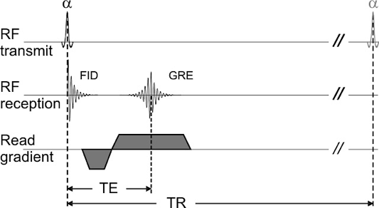
Gradient echoes ‑ also called gradient-recalled echoes (GRE), gradient-refocused echoes or field echoes – are the basis of many applications on modern MRI systems (1–4). Figure 1 shows the basic principle of such a GRE, where the free induction decay (FID) after radio-frequency (RF) excitation is measured. The most striking differences compared to a conventional spin echo sequence are, generally, the lacking refocusing pulse, the typically low excitation flip angle of α<90°, and the read gradient reversal.

A GRE sequence as outlined in Fig. 1 represents a quite “simple” form, implying a repetition time TR that is much longer than T1 and T2. Therefore, the transverse magnetization (Mxy) decays completely and the longitudinal magnetization (Mz) fully recovers until the next excitation pulse. Then, Mxy and, hence, the signal behavior and image contrast is dominated by the frequently introduced transverse decay time T2*:

$$ \frac{1}{T_2^*}=\frac{1}{T_2}+\frac{1}{T_2^{'}} \qquad [1]$$

As defined in Eq. [1], T2* is a combination of the tissue characteristic transverse relaxation time (T2) and a relaxation term, T2’, which reflects signal decay due to static field inhomogeneity and susceptibility effects. Note that it is always T2*<T2.

It has always been a necessity in MRI to actually shorten the acquisition time (TA) that is directly proportional to TR, which leads under certain circumstances to a dynamic magnetization equilibrium or steady state signal due to the incomplete T1 and T2 relaxation until the next RF excitation pulse.

Steady State Free Precession (SSFP)

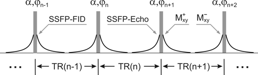
As originally introduced in 1958 by Carr (5) for NMR spectroscopy, a dynamic equilibrium or steady-state in the magnetization can be established by a train of RF excitation pulses interleaved by periods of ‘free precession’, commonly referred to as steady state free precession (SSFP) (see Fig. 2).

The quick succession of RF pulses prevents the magnetization from returning to thermal equilibrium and each RF pulse therefore acts on both remaining transversal and longitudinal magnetization generating rather complex patterns of spatial magnetization distribution even after a few RF pulses. Nevertheless, the magnetization between consecutive excitation pulses can reach a dynamic equilibrium, i.e. a steady state, if the following conditions are fulfilled, see (6,7):

• The dephasing from gradients (G) within TR, TR itself and the flip angle (α) must be constant.
• The phases (Φ) of the RF pulse must satisfy the equation: Φ_n = a + b×n +c×n²

Transition to steady state from thermal equilibrium (or any other magnetization prepared state) is completed after 5*T1, however, this is frequently not an acceptable waiting time. As a result, several preparation methods have been proposed to facilitate, enhance or smoothen this transition. In the following, we will assume that a steady state could have been established after sufficient RF pulses.

The class of fast GRE sequences that are based on the dynamic equilibrium effect of SSFP are commonly called SSFP sequences. Generally, the measured signal from such SSFP sequences will depend on relaxation (T1,T2) and on diffusion or flow effects, but also becomes a function of the repetition time (TR), the echo time (TE), the flip angle (α) and the RF pulse phase increment (Φ_n - Φ_n-1), and of the gradient switching pattern.

Basic SSFP Sequences

For incoherent SSFP imaging, the contribution from any residual transverse magnetization prior to the next excitation pulse is assumed to be zero, or spoiled. As a result, incoherent SSFP sequences show a pure T1 contrast, and the steady state signal immediately after the excitation pulse is given by

$$ M_{xy} = M_0 \frac{1-E_1}{1-E_1 \cos{\alpha}}\sin{\alpha} \quad , \quad E_1 \doteq \exp{(-TR/T_1)} \qquad [2] $$

Equation [2] is also known as the “Ernst equation” (8). However, the tricky part here is to get rid of all the transverse magnetization components prior to the next excitation pulse or to find a clever method to avoid any significant contribution in subsequent repetition periods.

The simplest way of efficient spoiling is a long enough waiting time but this is not very practical and a different spoiling strategy has to be used. An elegant and rather efficient approach is to adapt the phase of the RF excitation pulse Ф in every TR interval (c.f. Fig. 3a) to have a linear phase increment according to the formula

$$ \phi_n - \phi_{n-1} = \psi_0 + n \cdot \psi \qquad [3] $$

This method ‑ commonly referred to as RF spoiling (7,9,10) ‑ generates quadratically increasing phase offsets in the residual transverse magnetization. A proper choice of ψ (e.g., ψ = 50° or ψ = 117°) leads to a near complete destructive interference of all residual transverse magnetization components.

For SSFP, the dephasing from gradients must be constant and phase encoding gradients need to be rewinded ‑ a possible sequence diagram for the RF spoiled SSFP is shown in Fig. 3a. Asides, RF spoiling always comes with crusher gradients ‑ sometimes also (improperly) called spoiler gradients.

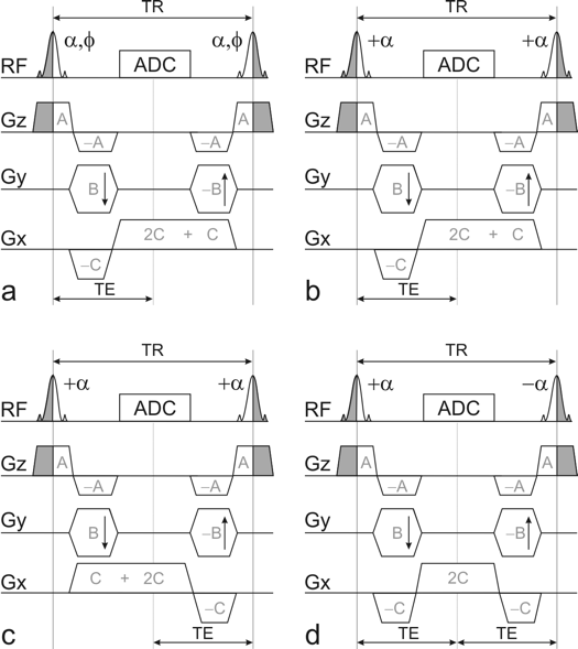
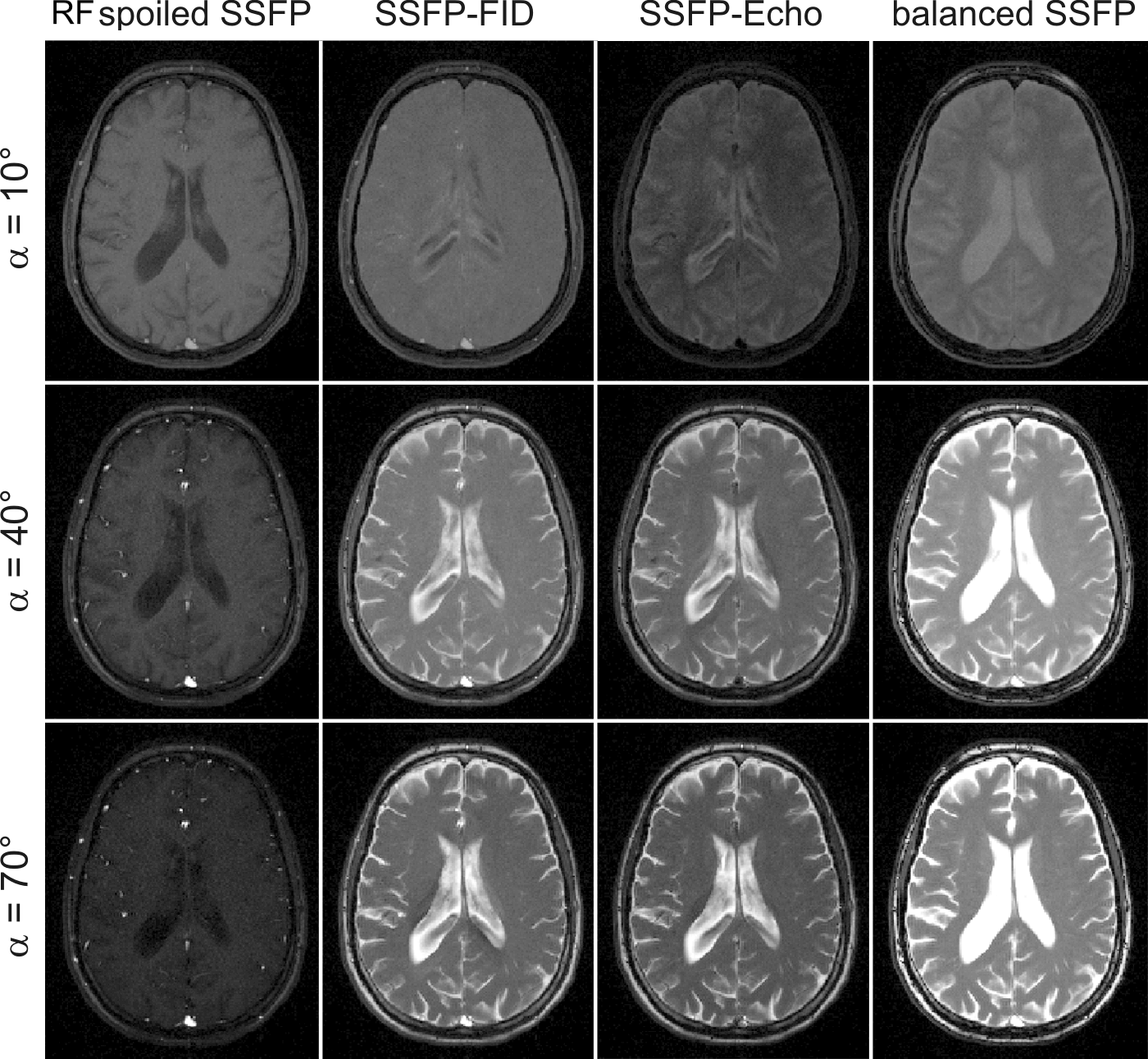
Figure 3 provides a general overview of four major types of SSFP sequences with corresponding contrast images shown in Figure 4. In fact, all four major types (RF spoiled SSFP, SSFP-FID, SSFP-Echo, balanced SSFP) can be regarded as a variant from a generic SSFP sequence. Their sole difference is whether the particular type of SSFP employs RF spoiling and crusher gradients in each case; however, the resulting signal behavior and image contrast is different.

Figure 3a displays the already discussed RF spoiled SSFP sequence (including a crusher gradient in the readout direction) that facilitates a dominant T1 contrast. Omitting RF spoiling but keeping the application of crusher gradients prior to the next excitation pulse, leads to the SSFP-FID sequence (Fig. 3b). A time-reversal of the readout gradient as displayed in Fig. 3c leads to the SSFP-Echo sequence.

Finally, balanced SSFP refers to an acquisition scheme as given in Fig. 3d, where all gradients have a zero net area within any TR (= balanced); and any residual phase accruals within any TR are therefore closely related to field inhomogeneities. As a result, balanced SSFP is prone to off-resonances that can lead to prominent signal voids or banding artifacts in regions of strong susceptibility variations and with poor shimming.

Acknowledgements

References

1. Haase A, Frahm J, Matthaei F, Hänicke W, Merboldt KD. FLASH imaging. Rapid NMR imaging using low flip-angle pulses. J Magn Reson 1986;67:258–266.

2. Markl M, Leupold J. Gradient echo imaging. J Magn Reson Imaging 2012;35:1274–1289.

3. Bieri O, Scheffler K. Fundamentals of balanced steady state free precession MRI. J Magn Reson Imaging 2013;38:2–11.

4. Hargreaves B. Rapid gradient-echo imaging. J Magn Reson Imaging 2012;36:1300–1313.

5. Carr HY. Steady-State Free Precession in Nuclear Magnetic Resonance. Phys Rev 1958;112:1693.

6. Sobol WT, Gauntt DM. On the stationary states in gradient echo imaging. J Magn Reson Imaging 1996;6:384–98.

7. Zur Y, Wood ML, Neuringer LJ. Spoiling of transverse magnetization in steady-state sequences. Magn Reson Med 1991;21:251–263.

8. Bernstein MA, King KF, Zhou XJ. Handbook of MRI Pulse Sequences. New York: Elsevier Academic Press; 2004.

9. Crawley AP, Wood ML, Henkelman RM. Elimination of transverse coherences in FLASH MRI. Magn Reson Med 1988;8:248–260.

10. Duyn JH. Steady state effects in fast gradient echo magnetic resonance imaging. Magn Reson Med 1997;37:559–568.