Basics of Transmission Lines & Power Transfer
1University of Alberta, Edmonton, AB, Canada
Synopsis
This lecture covers the basic concepts of RF power transfer over transmission lines. Tools such as scattering parameters and the Smith chart are also discussed.
Introduction
Transmission lines are used in MR systems to carry RF power (excitation) and signal (reception) to and from the RF coil and spectrometer. Maximizing the efficiency of these connections is important to achieving the best RF performance.Lumped Circuits and Matching Conditions
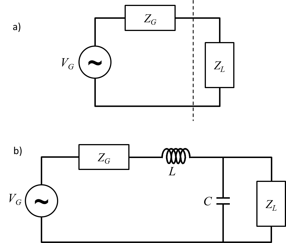
Lumped circuits are a simplification of physical circuits whereby it is assumed that no fields exist outside the lumped elements and that voltage anywhere along a connection is constant. At radio frequencies (RF) circuits are typically analyzed using phasor notation, which means that voltages and currents vary sinusoidally in time and are represented by complex numbers having the quantity’s corresponding phase and magnitude. Circuit elements are represented by complex impedances ($$$Z$$$), or their inverse, admittances ($$$Y$$$). The simple lumped circuit shown in Figure 1a represents a generator, with RF voltage $$$V_G$$$ and internal impedance $$$Z_G$$$, that feeds power to a load impedance $$$Z_L$$$. It may be shown that maximum power is transferred to the load if $$$Z_L=Z_G^*$$$ (i.e., conjugate match). With few exceptions (e.g., noise matching to achieve optimal amplifier noise figure), matching for maximum power transfer is the condition that is usually desired for both power and signals. Figure 1b shows that same circuit with the addition of parasitic elements (inductance and capacitance) corresponding to a connection of non-negligible length (but still $$$\ll$$$ the wavelength) between generator and load. The presence of these parasitic elements changes the matching conditions and therefore the amount of power transferred between generator and load.Uniform Transmission Lines
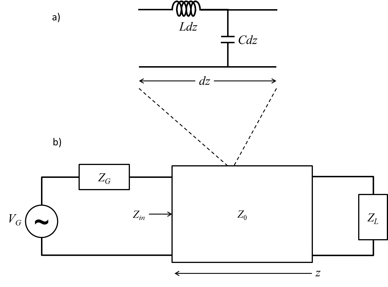
Connections that exceed or approach a substantial fraction of a wavelength are made using uniform transmission lines, such as coaxial cables, whose cross-sectional geometry does not change along the length. This allows the length of the transmission line to be divided into infinitesimal sections $$$dz$$$ (Figure 2a), from which the telegrapher equations are derived using Kirchhoff’s laws [1]:
$$\frac{{dV\left(z\right)}}{{dz}}=-i\omega LI\left(z\right)$$
$$\frac{{dI\left(z\right)}}{{dz}}=-i\omega CV\left(z\right).$$
Here $$$L$$$ and $$$C$$$ represent, respectively, the inductance and capacitance per unit length of the transmission line. Differentiating these equations and substituting for the first derivatives yields
$$\frac{{{d^2}V\left(z\right)}}{{d{z^2}}}+{\omega ^2}LCV\left(z\right)=0$$
$$\frac{{{d^2}I\left(z\right)}}{{d{z^2}}}+{\omega^2}LCI\left(z\right)=0,$$
which are one-dimensional forms of the Helmholtz equation (phasor wave equation) and thus describe waves that propagate with phase velocity $$${v_p}=1/\sqrt{LC}$$$ in either direction:
$$V\left(z\right)=V_0^+{e^{-i\omega z/{v_p}}}+V_0^-{e^{i\omega z/{v_p}}}$$
$$I\left(z\right)=I_0^+{e^{-i\omega z/{v_p}}}+I_0^-{e^{i\omega z/{v_p}}}.$$
For each direction the ratio of voltage and current is a constant known as the characteristic impedance
$${Z_0}=\frac{{V_0^+}}{{I_0^+}}=\frac{{V_0^-}}{{I_0^-}}=\sqrt{\frac{L}{C}},$$
and allows the general solution to be written as a function of only voltage or current waves. Terminating the transmission line with a load impedance $$$Z_L$$$ (Figure 2b) imposes a boundary condition at $$$z=0$$$ and thus a relationship between incident and reflected waves
$$V_0^-=\frac{{{Z_L}-{Z_0}}}{{{Z_L}+{Z_0}}}V_0^+={\rm{\Gamma }}V_0^+,$$
where $$$\Gamma$$$ is known as the voltage reflection coefficient and $$$\left|{\rm{\Gamma }}\right|\le1$$$ (for a passive $$$Z_L$$$). The condition for maximum power transfer to the load is $$$\Gamma=0$$$, i.e., $$$Z_L=Z_0$$$. If the reflection coefficient is known the impedance is calculated as
$$\frac{{{Z_L}}}{{{Z_0}}}=\frac{{1+{\rm{\Gamma}}}}{{1-{\rm{\Gamma}}}},$$
where we have explicitly normalized it relative to $$$Z_0$$$. It may be shown that at other points ($$$z$$$) along the transmission line the phase of the reflection coefficient changes in proportion to the length
$${\rm{\Gamma }}\left(z\right)={\rm{\Gamma}}\left(0\right){e^{-2i\omega z/{v_p}}},$$
making a full rotation in a distance of one half wavelength. Consequently, the impedance of the load is transformed by the line according to
$$\frac{{{Z_{in}}}}{{{Z_0}}} = \frac{{1 + {\rm{\Gamma }}\left( 0 \right){e^{ - 2i\omega z/{v_p}}}}}{{1 - {\rm{\Gamma }}\left( 0 \right){e^{ - 2i\omega z/{v_p}}}}}.$$
To obtain admittances the inverse of this equation is used.
Scattering Parameters
Scattering (or S) parameters [1] are an extension of the definition of reflection coefficient to devices that have more than one connection (port), e.g., transmission lines, amplifiers, attenuators, power splitters, circulators, T/R switches, etc. The reflected waves ($$$V_i^ - $$$) are obtained from the incident waves ($$$V_i^ +$$$) by multiplication with the S matrix
$$\left[ {\begin{array}{*{20}{c}}{V_1^ - }\\{V_2^ - }\end{array}} \right] = \left[ {\begin{array}{*{20}{c}}{{S_{11}}}&{{S_{12}}}\\{{S_{21}}}&{{S_{22}}}\end{array}} \right]\left[ {\begin{array}{*{20}{c}}{V_1^ + }\\{V_2^ + }\end{array}} \right].$$
Each element of the S matrix represents the reflected wave when only one port is driven and all ports are matched. If this condition is satisfied then the diagonal elements of S are the actual reflection coefficients seen at the respective ports. The off-diagonal elements are coupling (transmission) coefficients between ports. Scattering parameters are provided for most RF devices or measured using a vector network analyzer (VNA).
Smith Chart
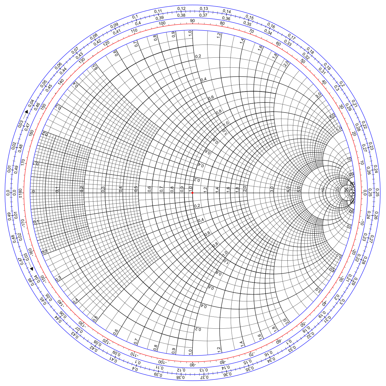
The Smith chart (Figure 3) is a convenient graphical tool that represents the coordinate transformation between $$$\Gamma$$$ inside the unit circle and the normalized impedance ($$$Z/Z_0$$$) or admittance ($$$YZ_0$$$). The transformed impedance is obtained graphically as follows [2]:
- find the normalized load impedance in curvilinear coordinates and identify the corresponding magnitude of $$$\Gamma$$$ (e.g., set the radius of a compass)
- starting from that point, use the compass to draw an arc of a circle (centered at the origin) for a total rotation equal to half the number of wavelengths ($$$\omega z/{v_p}$$$)
- read the normalized load impedance in curvilinear coordinates at the end of the arc.
With this procedure it is readily observed that a half-wavelength line (or any multiple thereof) transforms any impedance into itself, which is useful when matching to $$$Z_0$$$ is not desired or practical. A quarter-wave line (plus any number of half wavelengths) inverts the normalized impedance
$$\frac{{{Z_{in}}}}{{{Z_0}}}=\frac{{{Z_0}}}{{{Z_L}}},$$
and is used to perform impedance matching as well as to transform an infinite impedance to a short and vice versa.
The Smith chart also allows seeing the effect (on the reflection coefficient) of adding impedances to the load. Matching (achieving $$$\Gamma=0$$$) typically consists of adding reactances in series (parallel) to follow the constant-resistance (-conductance) circles on the Smith chart. Figure 10.2 of Ref. 2 illustrates the range of use of the 8 possible L-type matching networks.
Matching Circuits and Baluns
In addition to L-type matching networks, in MR applications it is common to find $$$\Pi$$$ and T networks [3] as well as lattice baluns [4]. The word balun is a portmanteau of balanced and unbalanced, which refer to whether the voltages on the conductors of the transmission line are symmetric (balanced) or relative to a ground conductor that is always at zero potential. Baluns are used often to allow a connection between a coaxial cable (unbalanced) and a coil that requires symmetric drive.Acknowledgements
NAReferences
- David M. Pozar, Microwave Engineering, Fourth Edition. 2012 Wiley.
- Phillip H. Smith, Electronic Applications of the Smith Chart, Second Edition. 2000 SciTech Publishing.
- Reykowski A, Wright SM, Porter JR. Design of matching networks for low noise preamplifiers. Magn Reson Med 1995;33:848–852.
- Frankel S. Reactance networks for coupling between unbalanced and balanced circuits. Proc IRE 1941;29:486–493.
Figures