Synopsis

Compressed-sensing (CS) MRI is frequently based on the minimization of an objective function consisting of the $$$\ell_1$$$-norm of a sparse image representation and the total variation (TV) of the image. Various definitions of the TV exist (isotropic/anisotropic; first-order/second-order/combined; and, particularly for complex-valued image data, several ways of dealing with real and imaginary parts of the image). The purpose of this abstract is to explain these variants, to provide implementation details, and to compare several variants with respect to CS reconstruction.

Introduction

Over the last years, compressed-sensing (CS) MRI has found considerable interest for accelerated MR image acquisition based on sparse k-space sampling^1–4. Frequently, the compressed sensing reconstruction can be expressed as minimization of a an objective function $$||\Psi m||_1+\alpha \mathrm{TV}(m)$$ consisting of the $$$\ell_1$$$-norm of a sparse representation $$$\Psi m$$$ (such as a wavelet transform) of the (complex-valued) image $$$m$$$ and of a total variation (TV) term (weighted by the factor $$$\alpha$$$); this objective function is minimized under the data-consistency constraint $$||\cal{F}_u m–y||_2<\epsilon,$$ where $$$\cal{F}_u$$$ is the undersampled Fourier transform and $$$y$$$ the measured k-space data².

In particular for complex-valued image data, several variants and definitions of the TV exist. The purpose of this abstract is to explain these variants, to provide implementation details, and to compare several variants with respect to CS reconstruction.

Theory

The (2D) first-order TV can be expressed as the $$$\ell_1$$$-norm of the horizontal ($$$D_x$$$) and vertical ($$$D_y$$$) finite differences, which can be combined either isotropically $$\mathrm{TV_{iso}}(m)=\Big|\Big|\sqrt{(D_x m)^2+(D_y m)^2}\Big|\Big|_1$$ (with pixelwise square and square-root operations) or anisotropically $$\mathrm{TV_{aniso}}(m)=||D_x m||_1+||D_y m||_1.$$

For complex image data $$$m=u+iv$$$, the total variation can be calculated (1) separately for the real and imaginary part $$\mathrm{TV_{sep}}(m)=\mathrm{TV}(u)+\mathrm{TV}(v),$$ (2) for the magnitude of the data $$\mathrm{TV_{mag}}(m) = \mathrm{TV}(|m|),$$ or (3) using complex finite differences, e.g. $$\mathrm{TV_{cplx,aniso}}(m)=||D_x (u + iv)||_1 +||D_y (u+iv)||_1,$$ where magnitudes are calculated as part of the $$$\ell_1$$$-norm calculation.

The second-order TV includes finite differences of higher order⁵: $$$D_{xx}, 2D_{xy}, D_{yy}$$$, which can be combined exactly as the first-order differences described above. First-order and second-order TV can be applied either alone or in a weighted combination described by weights $$$(\beta, 1-\beta)$$$.

Methods

CS and in particular the TV calculation were implemented in Python 3 (using the PyWavelets package and the conjugate-gradient minimizer scipy.optimize.fmin_cg) guided by the Matlab implementation by Lustig et al.⁶ (i.e., combining a Daubechies wavelet sparsifying transform and a TV approach; data reconstruction was implemented with Lagrange multipliers $$$\lambda_1=0.003, \lambda_2=0.002$$$ for wavelet and TV penalty, respectively).

TV derivatives (i.e. gradient functions of the TV as required for the iterative conjugate-gradient minimizer) with a smoothing parameter² $$$\mu=10^{-10}$$$ were also implemented for all variants. Python sourcecodes will be made publicly available in 2018.

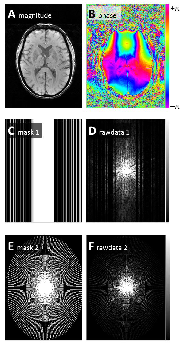
CS reconstruction was evaluated for a 2D slice of a brain gradient-echo image (TE=20 ms, TR=50 ms, matrix=320×240); retrospective undersampling of the k-space was performed with (a) linear variable-density random sampling in phase-encoding direction (2.33fold undersampling; full sampling of k-space center, sparse Poisson-disk sampling of the periphery) and (b) radial sampling (4.06fold undersampling with 80 spokes); cf. Fig. 1.

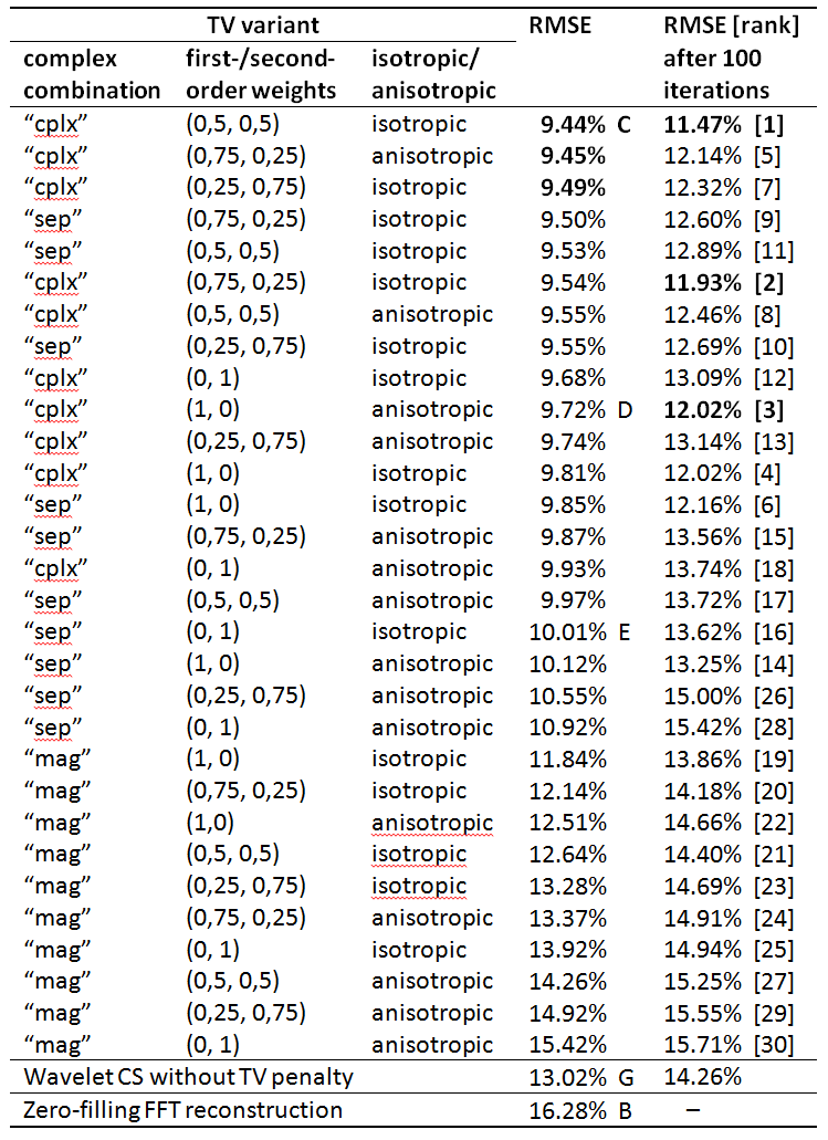
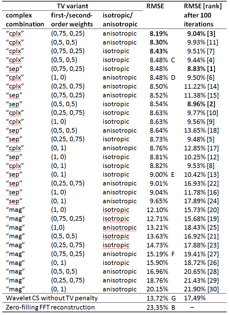
To illustrate the differences between the different TV implementations, CS reconstruction was performed for 30 variants of the TV combining all possibilities of: isotropic/anisotropic; $$$\mathrm{TV_{sep}}(m)/\mathrm{TV_{mag}}(m)/\mathrm{TV_{cplx}}(m)$$$; and 1st-order/2nd-order TV combinations $$$(\beta, 1-\beta)= (1,0), (0,1), (0.5,0.5), (0.75,0.25), (0.25,0.75)$$$, yielding the 2×3×5 = 30 variants.

The results of each iterative CS reconstruction after 100 and 2000 iterations were compared to the (complex) ground truth image (fully sampled Fourier reconstruction) by calculating the relative root-mean-square error (RMSE) based on the magnitude of the complex differences.

Results

All TV variants were implemented in Python with comparable computational efficiency; TV derivatives were verified by comparison to the numerically determined derivatives.

With 2.33fold linear undersampling (a), the relative RMSE of the zero-filling reconstruction was 16.3%; the RMSE of wavelet CS without TV penalty was 13.0%. With TV penalty, the resulting RMSE varied substantially (between 9.4% and 15.4%) depending on the TV variant as summarized in Table 1.

With 4.06fold radial undersampling (b), the relative RMSE of the zero-filling reconstruction was 23.4%; the RMSE of wavelet CS without TV penalty was 13.7%. With TV penalty, the resulting RMSE varied substantially (between 8.2% and 20.2%) depending on the TV variant as summarized in Table 2.

Best results were obtained for $$$\mathrm{TV_{cplx}}(m)$$$ with weighted combinations of 1st- and 2nd-order TV. Second or first-order TV alone resulted in worse RMSE values. No substantial difference was found between isotropic and anisotropic TV. The magnitude combination $$$\mathrm{TV_{mag}}(m)$$$ yielded clearly inferior results. $$$\mathrm{TV_{cplx}}$$$ and $$$\mathrm{TV_{sep}}$$$ performed similarly with a slight trend favoring $$$\mathrm{TV_{cplx}}$$$.

After only 100 iterations, a similar ranking of TV variants was obtained as after 2000 iterations; however, the RMSE values were about 10 to 40% higher than after 2000 iterations.

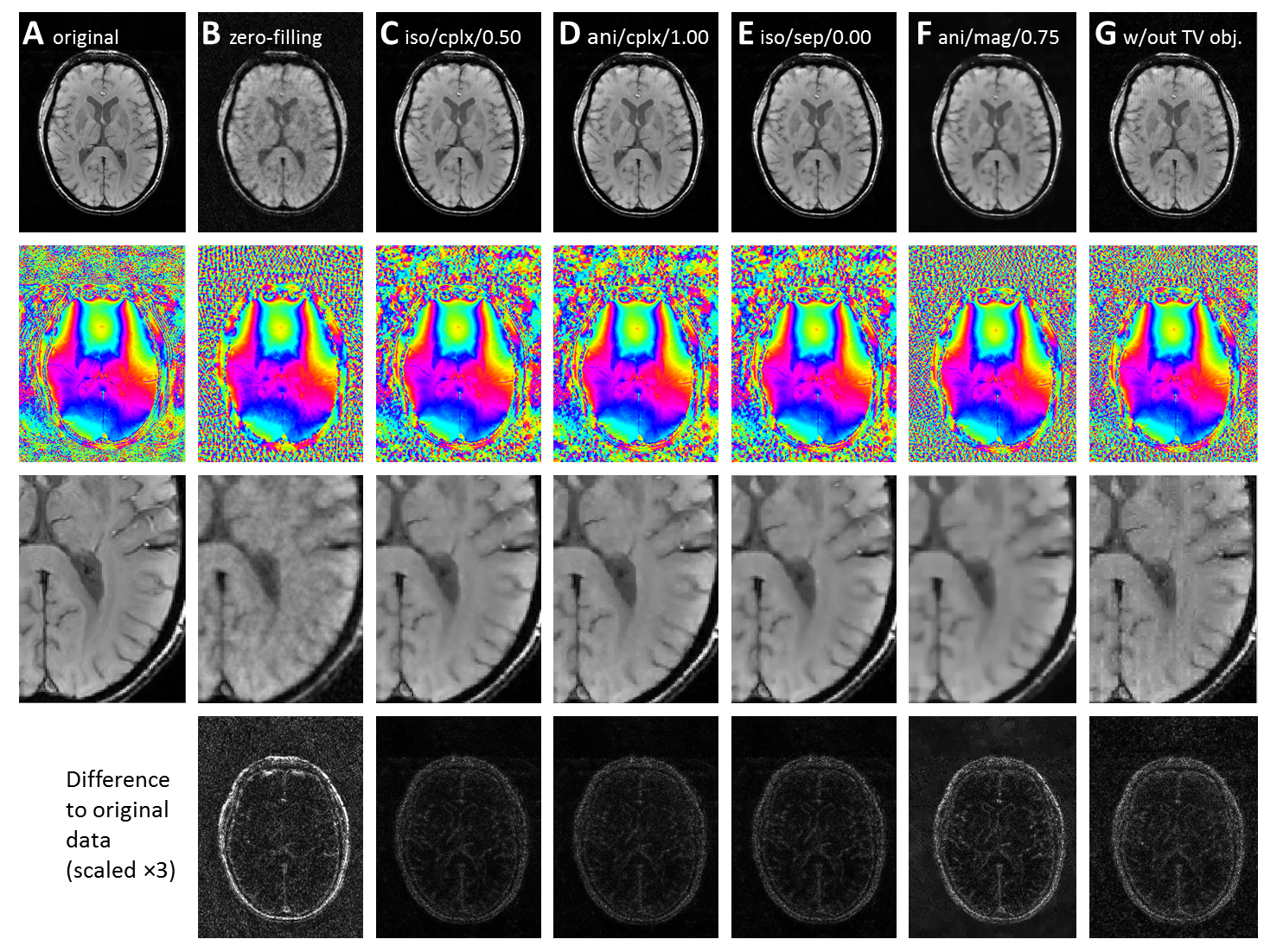
Representative examples of reconstructed images are shown in Figs. 2 and 3.

Conclusion

Acknowledgements

References

1. Candès EJ, Romberg J, Tao T: Robust uncertainty principles: Exact signal reconstruction from highly incomplete frequency information. Information Theory, IEEE Trans 2006;52(2):489–509.

2. Lustig M, Donoho D, Pauly JM. Sparse MRI: The application of compressed sensing for rapid MR imaging. Magn Reson Med. 2007 Dec;58(6):1182–1195.

3. Geethanath S, Reddy R, Konar AS, et al. Compressed sensing MRI: a review. Crit Rev Biomed Eng. 2013;41(3):183–204.

4. Zhao D, Du H, Han Y, Mei W. Compressed sensing MR image reconstruction exploiting TGV and wavelet sparsity. Comput Math Methods Med. 2014;2014:958671.

5. Lefkimmiatis S, Bourquard A, Unser M. Hessian-based norm regularization for image restoration with biomedical applications. Image Proc, IEEE Trans. 2012;21(3):983–995.

6. Lustig M et al. Sparse MRI. Available online at <http://people.eecs.berkeley.edu/~mlustig/Software.html>