5652
Geometry in MR Reconstruction1University College London, London, United Kingdom
Synopsis
Keeping track of positional information, from planning the position of a field of view, through to the final reconstructed image can be challenging. This educational poster highlights some of the issues and pitfalls in the acquisition and reconstruction process. Use of DICOM-style spatial referencing is encouraged and strategies for validation are presented.
Introduction
Maintaining correct geometrical information during reconstruction is important for surgery and radiotherapy applications, for consistent alignment when using multiple images, e.g. multi-parametric MRI, PET-MR, B0 distortion correction, for clarity in standards e.g. ISMRMRD1 and when comparing new reconstructions to clinical DICOMs. Correct handling can be challenging due to: conventions used in the Fast Fourier Transform, radiological image orientations, a requirement for square pixels and images and the ‘centre point’ falling on a voxel boundary for even-length arrays. We provide some clarity, guidance and suggestions for validation.DICOM
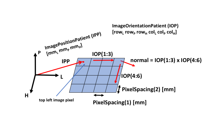
Figure 1 shows the DICOM convention for spatially referencing an image using the ImagePositionPatient (IPP) vector to a point, and ImageOrientationPatient (IOP) vectors along a row and column. This point and two vectors convention allows for easy manipulations of image data following the Fourier Transform, e.g. to display in a radiological orientation.
In multi-slice 2D imaging, the temporal order of slice acquisition can vary. When assembling a volume, slice positional order can be determined from the scalar product of the IPP vector with the slice normal (formed from the cross product of the row and column vectors).
Scanning Process
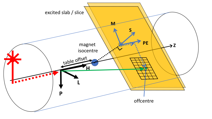
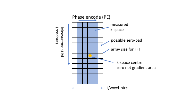
The initial laser positioning sets a point in the body and after planning, table movements mean this point may not coincide with the magnet isocentre (Figure 2). The position of the excited slice (2D) or centre of a slab (3D) is set by the RF excitation frequency and the slice select gradient which can have any angulation, achieved by combining physical X,Y and Z gradients. An entire slice/slab is excited, but filtering the received frequencies restricts the spatial extent in the frequency encode direction (M), and by changing the centre frequency, a desired offset in M is achieved. In the phase encode (PE) direction, linearly changing the acquired phase provides a PE offset of the image after Fourier Transform. These offsets may differ from the user-specified offset if a) a half-pixel shift is added in acquisition (to move the image ‘centre’ off a voxel boundary), or b) in-plane offcentres are not applied in acquisition, but achieved by shifting in post-processing, e.g. in the case of readout ramp sampling. The k-space origin is the point acquired when the net gradient area was zero. Zero-padding of k-space may be applied to adjust the reconstructed voxel size, typically to make it equal in M and PE directions (Figure 3). Shim fields may be defined in terms of X, Y and Z directions.Fourier Transform
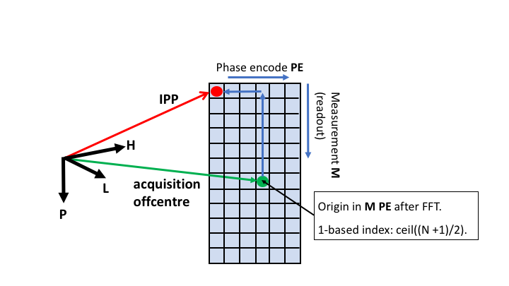
K-space to image space conversion uses the forward Fourier Transform ( –ve sign in the exponential). By convention, the FAST FT algorithm expects both input and output data to be half-shifted so that the origin is at the start of the array (not the centre). Shifting and inverse shifting operations are not identical for odd-sized arrays so should be applied in the correct order. In MATLAB the operation is img = fftshift( fft( ifftshift( kspace ))). Using 1-based indexing and after shifting, the origin is at array index: ceil((N+1)/2), see Figure 4.
Following FFT, any required image cropping, zero-padding, reflection or 90 degree rotations do not change the voxel size and spatial referencing is easily updated using the DICOM-style point and two vectors representation. For example, following a 90 degree counter-clockwise rotation, the new row vector is the old column vector, the new column vector is the negative of the old row vector and the new top left pixel is the old bottom left (whose 3D coordinates are easily calculated before the rotation using IPP and IOP vectors and voxel sizes).
Validation
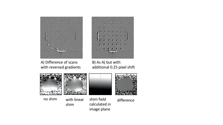
Geometrical handling can be checked by comparing reconstructions from scans acquired at multiple offsets, angulations, fat shift and phase encode directions. For test data, use spin echo sequences with high bandwidth (to reduce distortions), a power of 2 FOV, e.g. 256mm with 2mm voxel size and 128 acquisition and reconstruction matrices (if zero-padding is to be avoided), image near isocentre (to reduce the effects of gradient non-linearities) and ignore alignment differences near to susceptibility boundaries. Small structures within a phantom are useful. Comparison requires reslicing one reconstruction to the geometry of another reconstruction chosen as a reference, possibly from an alternative algorithm, e.g. a scanner DICOM. Residual distortion and intensity changes mean subtraction images need visual interpretation. Comparison with errors from an intentional sub-pixel offset can help to guide interpretation. Interpretation of X, Y and Z directions can be tested by acquiring a field map with zero shim and comparing to one after shims specified in X, Y, Z have been subtracted (Figure 5).Acknowledgements
Cancer Research UK A21099, UK EPSRC EP/P022200/1, EP/M022587/1.References
1. Inati et al MRM 77 p411 (2017). 10.1002/mrm.26089Figures