5633
Higher-order subspace denoising for improved multi-contrast imaging and parameter mapping1Electrical and Computer Engineering, University of Arizona, Tucson, AZ, United States, 2Department of Medical Imaging, University of Arizona, Tucson, AZ, United States
Synopsis
Multi-contrast image acquisitions are valuable for diagnostics but the scan time scales with the number of contrast images. Accelerated acquisitions are necessary for practical scan times and require the use of constrained reconstructions. Subspace-constraints, which constrain the multi-contrast data to lie in a low-dimensional subspace, are popularly used to reconstruct these datasets. Despite yielding good quality images at most imaging contrasts, these constraints create poor image quality at certain contrasts. We demonstrate that this is due to poor recovery of higher order subspace coefficients and present a model to enable high quality recovery of these coefficients and consequently the echo-images.
Introduction
Multi-contrast MRI is a valuable diagnostic tool. It involves the acquisition of a series of $$$N$$$ contrast-weighted images ($$$(\mathbf{X}_{n})^{N}_{n=1}$$$) (e.g. at different echo times (TEs) for T2 mapping or inversion times (TIs) for T1 mapping). These images are then fit to a suitable signal model to extract parameter maps. Accelerated data acquisition is necessary to achieve clinically acceptable scan times and requires the use of constrained image reconstruction1-6 to generate $$$\mathbf{X}_{n}$$$. A popular class of reconstruction methods are based on enforcing subspace constraints and include methods like k-t PCA3 and its regularized variants4-6. The subspace constraint forces the $$$N$$$-dimensional contrast data into a $$$K$$$-dimensional subspace ($$$K<<N$$$) and acts as a hard rank constraint. Despite yielding high quality parameter maps, these models are known to create poor quality contrast images at early TEs (or TIs)6 which typically have high SNR. We show that this is further exacerbated due to the poor signal recovery of higher-order subspace coefficient images and present an approach that allows the recovery of these coefficients and, consequently, $$$\mathbf{X}_{n}$$$ and the corresponding parameter maps.Reconstruction models
The measured data can be related to $$$\mathbf{X}_{n}$$$ as follows: $$$\mathbf{Y=E(X)}$$$ where $$$\mathbf{X}_{M \times N}$$$ ($$$M$$$ spatial pixels) is a matrix with $$$\mathbf{(X}_{n})^{N}_{n=1}$$$ as its columns. A subspace-constraint for $$$\mathbf{X}$$$ takes the following form: $$$\mathbf{X} \approx \mathbf{\alpha}_{M \times K} \mathbf{\phi}_{K \times N}$$$ where $$$\mathbf{\phi}$$$ maps the $$$K$$$-dimensional subspace coefficients $$$\mathbf{\alpha}$$$ back to the $$$N$$$-dimensional contrast space. Subspace-constrained reconstruction takes the following general form: $$\min_\alpha\frac{1}{2}||\mathbf{Y}-\mathbf{E(\alpha\phi)}||_2^2+\lambda\mathbf{R(\alpha)}$$
When no additional regularization is used, this reconstruction is the same as k-t PCA3,4. Joint-sparsity (JS) constraints were used in4 while locally low rank (LLR) regularization was used in6 to augment subspace constraints. The regularizer in the JS model is $$$\mathbf{R(\alpha)}=||D_{x}\mathbf{\alpha}||_{2,1}+||D_{y}\mathbf{\alpha}||_{2,1}$$$ where $$$D_{x}$$$ are $$$D_{y}$$$ are the horizontal and vertical finite difference operators that operate on all the subspace images and $$$||.||_{2,1}$$$ is the mixed $$$\ell_2/\ell_1$$$ norm. The LLR model uses the nuclear norm, $$$||.||_{*}$$$, as a surrogate for rank and is defined as: $$$\mathbf{R(\alpha)}=\sum_{j}||T_{j}{\alpha}||_{*}$$$ where $$$T_{j}$$$ is an operator that extracts the relaxation (subspace) signals from a small spatial patch about the spatial pixel $$$j$$$ and orders the contrast signals from the patch into a matrix.
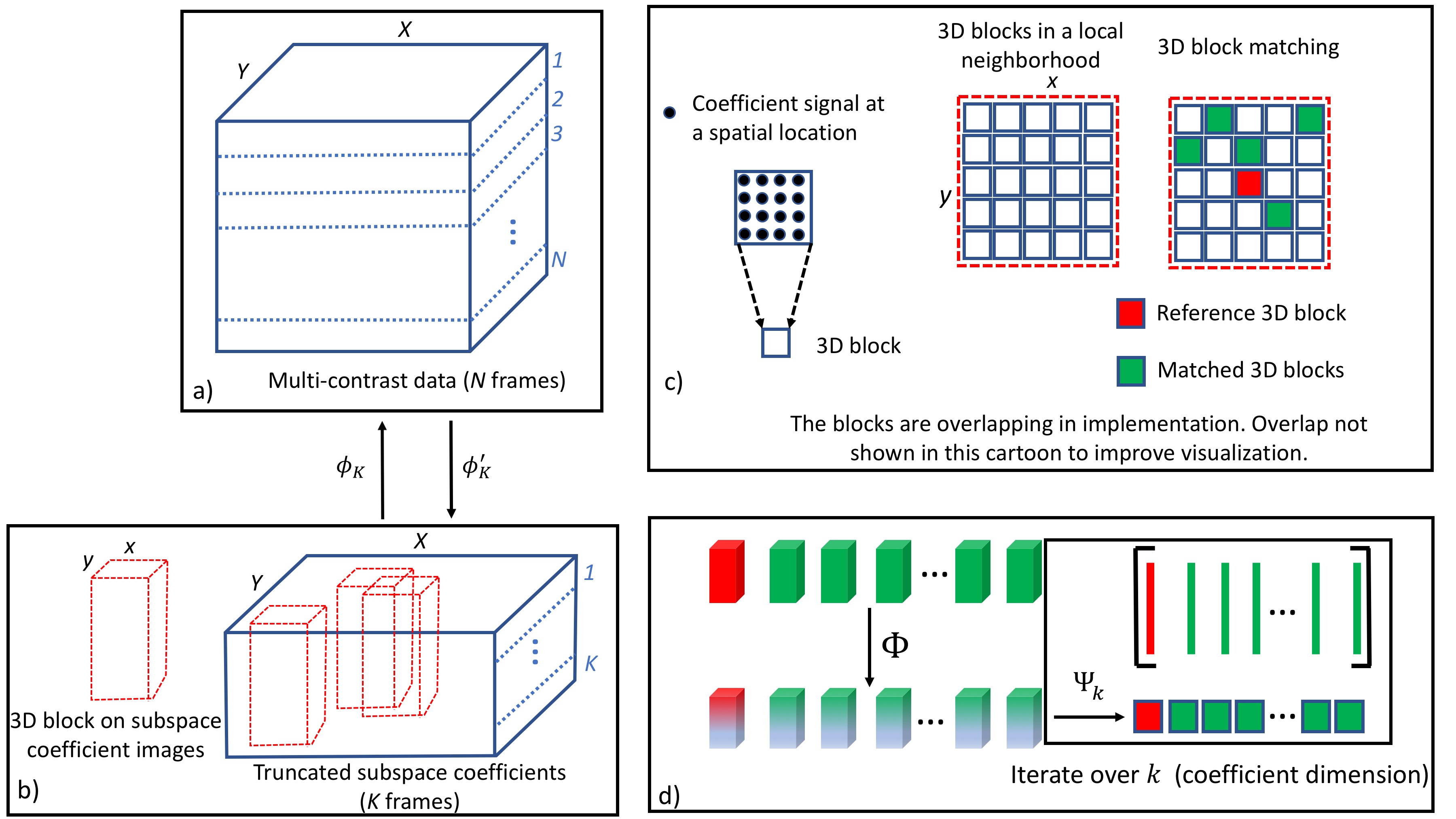
We propose a regularization operator built on 3D block matching (BM). For a reference 3D block (3DB), the BM algorithm identifies the L-nearest 3DBs in a local neighborhood. For the ensemble of patches, the regularization operator is defined as: $$\mathbf{R(\alpha)}=\sum_{j}\sum_{k}||\Psi_{k}(\Phi(R_{j}{\alpha}))||_{*}$$
The operator $$$R_{j}({\alpha})$$$ extracts the L-nearest (in $$$\ell_2$$$ sense) 3DBs for a reference 3DB indexed by $$$j$$$ using the BM algorithm. $$$\Phi(R_{j}({\alpha}))$$$ applies a temporal transform across the extracted 3DBs. We use the SVD algorithm to allow this transform to be data driven. $$$\Psi_{k}(.)$$$ extracts the spatial patches from the $$$k^{th}$$$ coefficient dimension and orders these as columns in a matrix which are then constrained with the nuclear norm. Note that the ensemble of 3DBs and the coefficient dimension are indexed by $$$j$$$ and $$$k$$$, respectively. The BM step makes this approach a form of non-local rank (NLR) constraint on transform domain data. Therefore, the method is named NLR3D. A cartoon illustrating subspace-constraint and the working of the proposed model is presented in Figure 1.
Methods
The proposed method was tested on data acquired with a radial fast spin echo sequence on a 3T Siemens Skyra scanner on brain and knee datasets. Fully sampled scans were retrospectively undersampled to simulate acceleration and to allow the generation of a reference dataset. Performance was evaluated using normalized mean squared error (NMSE). The subspace basis was generated using a library of training curves using the Slice-Resolved-Extended-Phase-graph (SEPG) model7 and SVD5-6. Reconstructed images are used to generate T2 maps and I0 (TE=0ms) maps using VARPRO8.Results
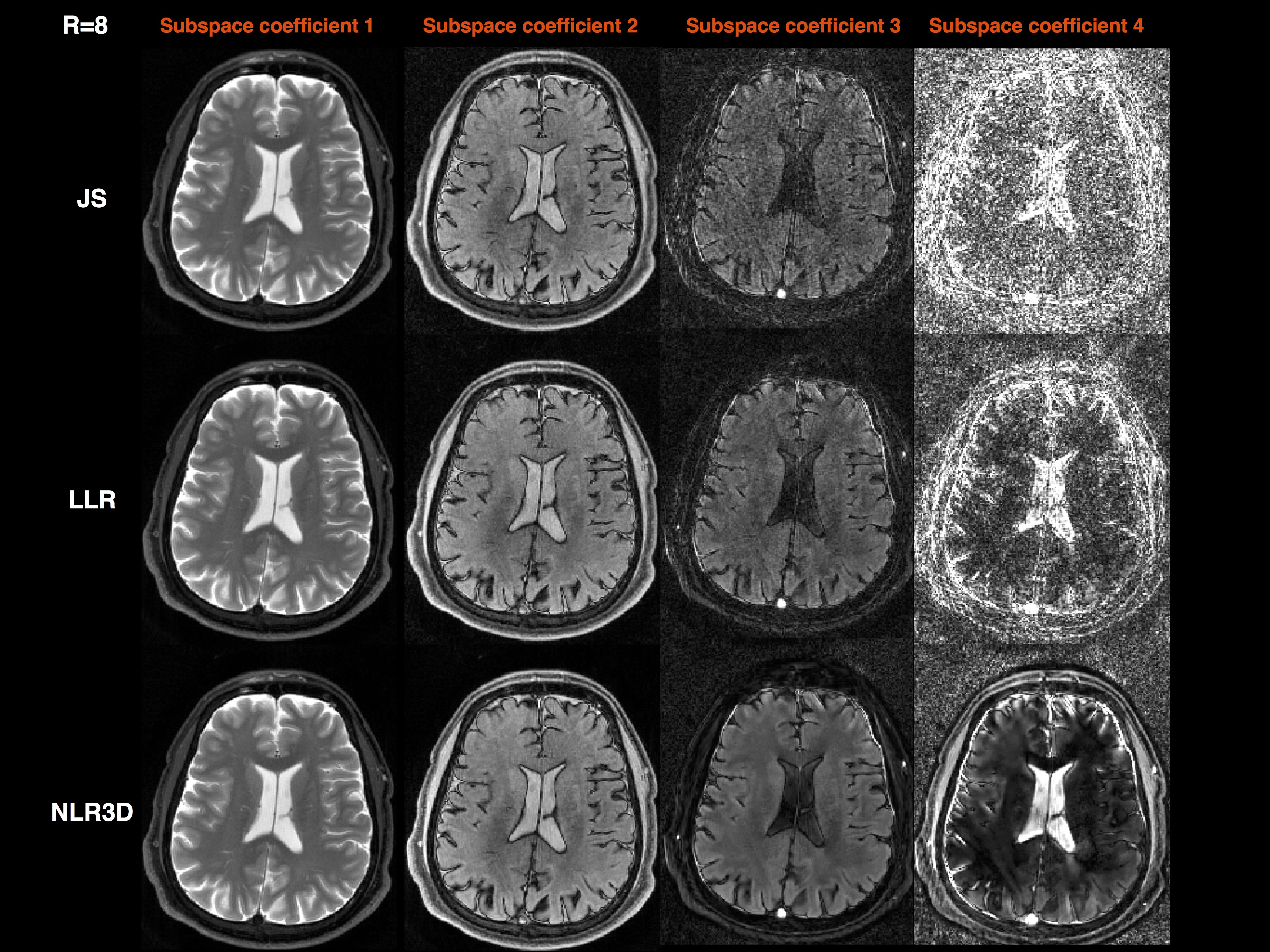
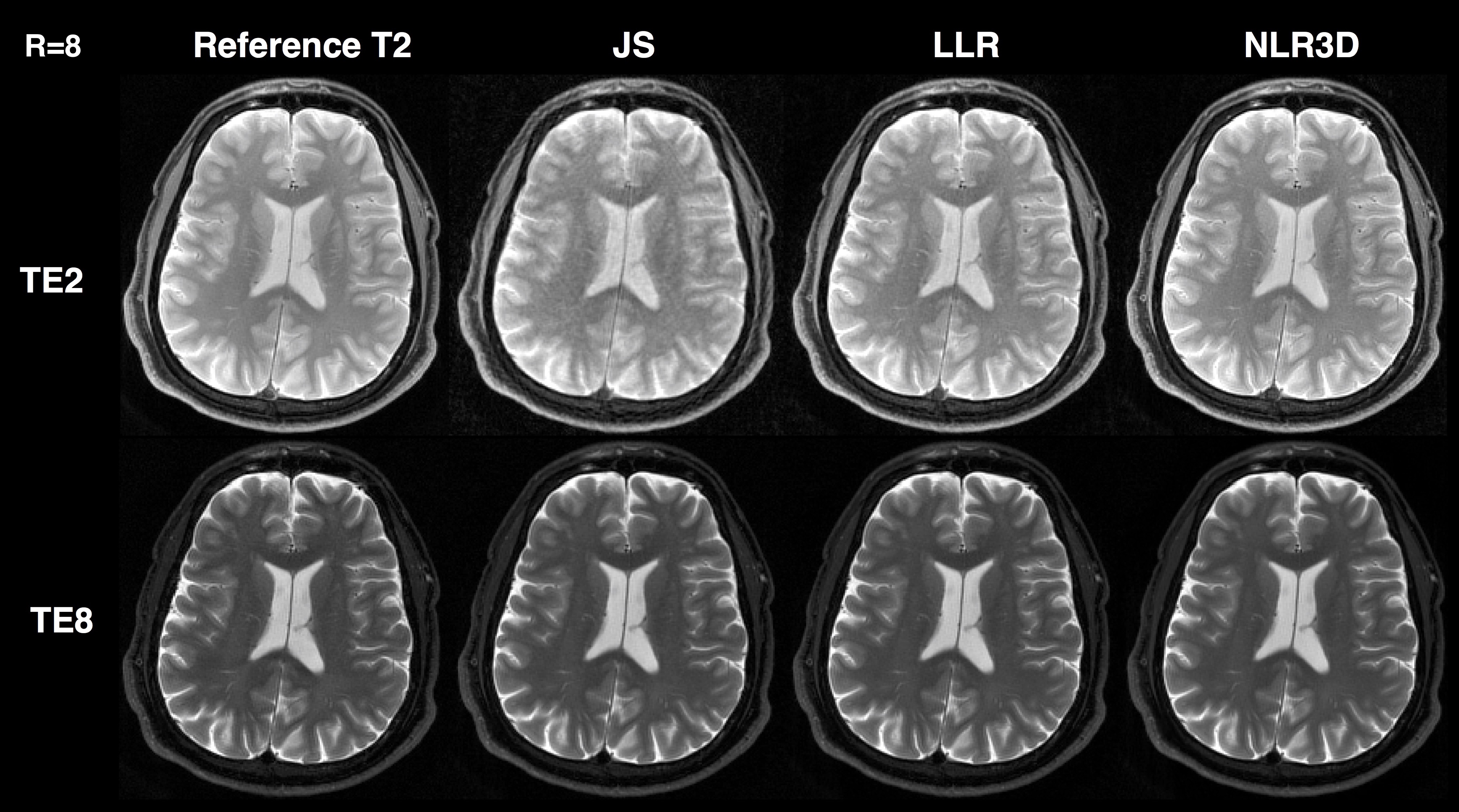
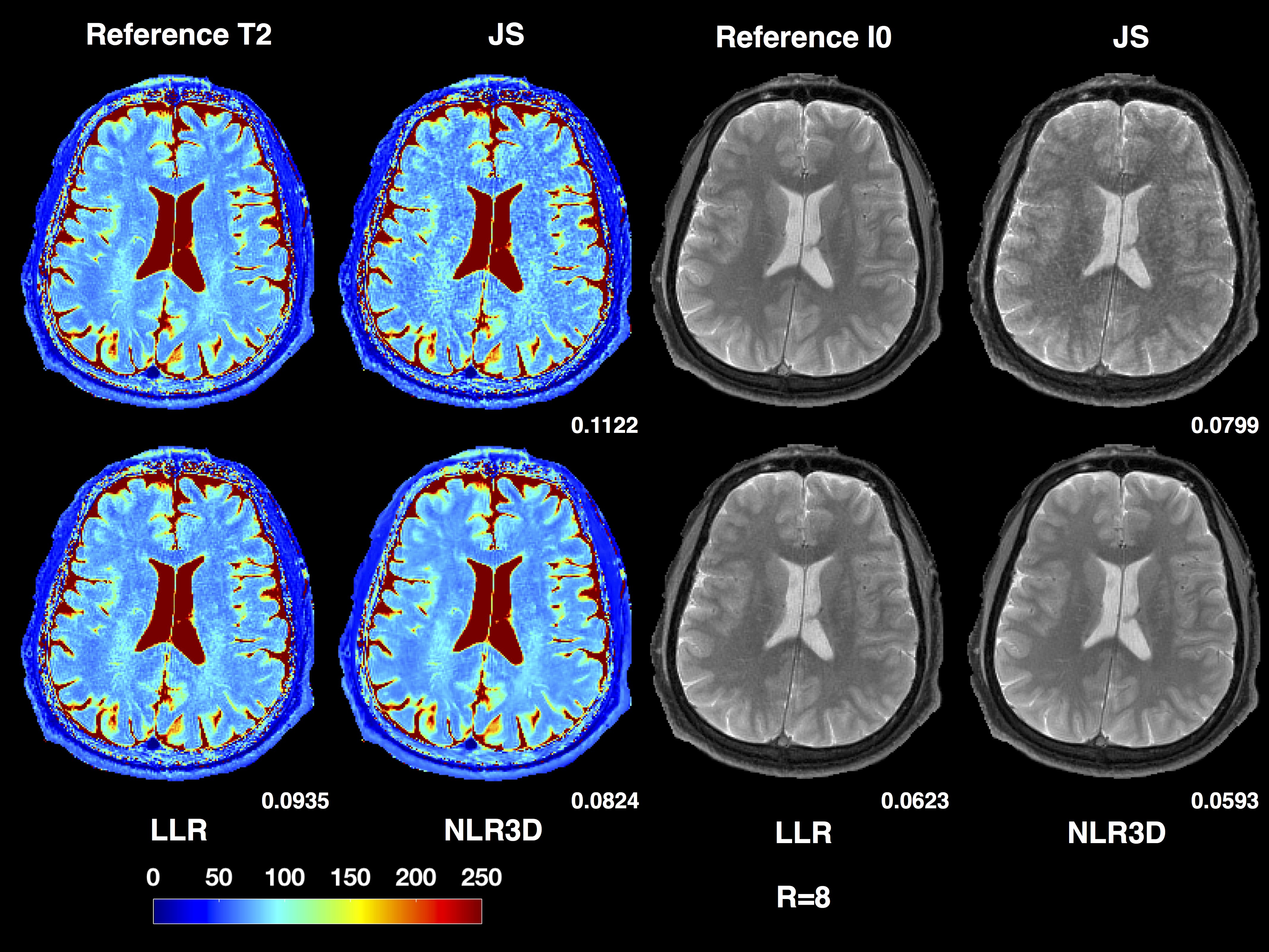
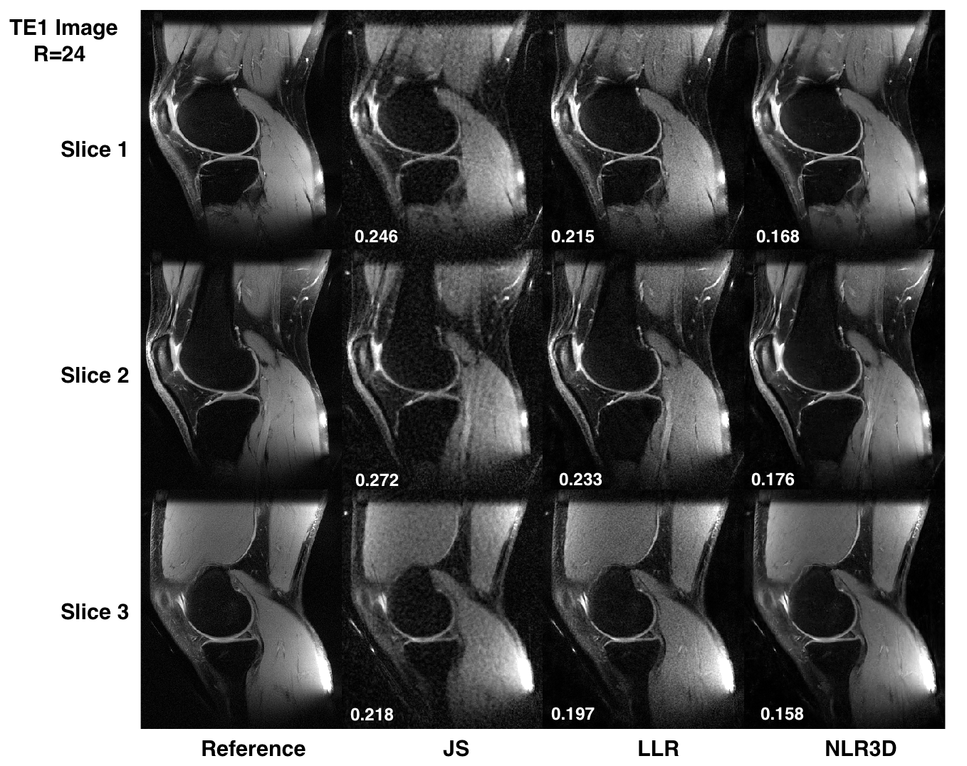
Figure 2 shows the subspace coefficients for the brain dataset for $$$N$$$=16 and $$$K$$$=4. Note the significantly improved recovery of higher-order coefficients with NLR3D. Figure 3 shows representative early-TE (TE2) and mid-TE (TE8) brain images generated from the subspace coefficients in Figure 2. Figure 4 shows the brain T2 and I0 maps corresponding to the results in Figures 2,3 with NMSE values reported on the bottom right of the maps. Figure 5 shows the TE=11ms image (proton-density weighted) from the knee dataset together with NMSE values for each reconstruction.Discussion and Conclusion
Subspace-constrained reconstructions are a powerful class of models that can enable high quality imaging. However, they can suffer from poor recovery of some temporal frames which leads to poor parameter mapping performance. The proposed model, NLR3D, can significantly reduce artifact in higher-order subspace coefficients leading to improved multi-contrast imaging and parameter mapping.Acknowledgements
The authors would like to acknowledge support from the Arizona Biomedical Research Commission (Grant ADHS14-082996) and the Technology and Research Initiative Fund (TRIF) Improving Health Initiative.References
[1] Bilgic B, Goyal VK, Adalsteinsson E. Multi-contrast reconstruction with Bayesian compressed sensing. MRM, 2011, 66, 1601– 1615.
[2] Velikina J, Alexander AL, Samsonov A. Accelerated MR parameter mapping using sparsity-promoting regularization in parametric dimension. MRM, 2013, 70, 1263-1273.
[3] Petzschner FH, Ponce IP, Blaimer M, Jakob PM, Breuer FA. Fast MR parameter mapping using k-t principal component analysis. MRM, 2011, 66, 706–716.
[4] Zhao B, Lu W, Hitchens TK, Lam F, Ho C, Liang Z-P. Accelerated MR parameter mapping with low-rank and sparsity constraints. MRM, 2014, 74, 489-498.
[5] Huang C, Graff CG, Clarkson EW, Bilgin A, Altbach MI. T2 mapping from highly undersampled data by reconstruction of principal component coefficient maps using compressed sensing. MRM, 2012, 67, 1355–1366.
[6] Tamir JI, Uecker M, Chen W, Lai P, Alley MT, Vasanawala SS, Lustig M. T2 shuffling: Sharp, multicontrast, volumetric fast spin-echo imaging. MRM, 2016, 77, 180-195.
[7] Lebel RM, Wilman AH. Transverse relaxometry with stimulated echo compensation. MRM, 2010, 64, 1005–1014.
[8] Golub G, Pereyra V. Separable nonlinear least squares: the variable projection method and its applications. Inverse Problems, 2003,19, R1–R26.
Figures