5599
Helmholtz Inversion Using Unconstrained Optimization for MR Elastography1Department of Radiology, The Ohio State University Wexner Medical Center, Columbus, OH, United States, 2Department of Biomedical Engineering, The Ohio State University, Columbus, OH, United States
Synopsis
MR elastography (MRE) is a phase-contrast MR technique in which the shear stiffness of soft tissues can be estimated. Helmholtz equation-based inversion is used to obtain stiffness of interest from MRE measurements. It is challenging to accurately estimate stiffness due to the presence of noise. In this work, an inversion method based on unconstrained optimization has been proposed where noise is reduced from the measured data while the sparsity of stiffness map in wavelet domain is being explored. Results demonstrated that optimization yielded more accurate stiffness estimation with lower root-mean-square error and lower maximum error when compared to local-frequency estimation.
Introduction
MR elastography (MRE) is a phase-contrast based MR technique through which the shear stiffness of soft tissues can be estimated [1-3]. To obtain a desired stiffness map from the acquired MRE data, an inversion algorithm based on Helmholtz equation is used [4-5]. However, correctly estimating shear stiffness can be challenging under the presence of noise because of the noise amplification resulted by the Laplacian operation within the Helmholtz equation. Local-frequency estimation (LFE) is an inversion method known to be robust to noise. However, it usually yields estimation errors around edges [2]. In this work, an inversion method based on unconstrained optimization has been proposed where noise is reduced from the measured data, while the sparsity of stiffness map in wavelet domain is being explored.Methods
Theory
The cost function of the above-mentioned optimization problem is
J(u, μ) = argmin||c * $$$\nabla$$$2u * μ - u||2 + λ1 ||u - u0||2 + λ2 ||ψ(μ)||1,
where $$$\nabla$$$2 is the Laplacian operator, c=-1 / (ρ ω2), ω is the angular mechanical frequency, μ is the stiffness of interest, u is the pursued displacement (less noisy), u0 is the measured displacement (noisy) from acquired MRE data, ψ is wavelet transform and λ1, λ2 are regularization coefficients.
The first term guarantees data fidelity when it is minimized since it describes the physical relationship between tissue displacement and its stiffness (i.e., the Helmholtz equation). The second regularization term allows the pursued displacement to deviate from the noisy displacement measured from phase images. The third regularization term ensures the sparisty of stiffness map in wavelet domain. Applied together, both regularization terms can effectively de-noise the measured displacement without blurring object’s edge and thus potentially generate more accurate stiffness maps. To solve this optimization problem, a balanced fast iterative/shrinkage thresholding algorithm (bFISTA) and the least-square method (LSQR) were used in optimizing the cost function [6-7].
Simulated Data and Physical Phantom Measurements
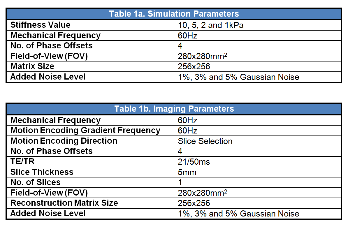
A four-band phantom with stiffness values of 10, 5, 2 and 1kPa was simulated in this study. Single-directional planar waves were assumed throughout the simulation. Additionally, MRE measurements were performed on a cylindrical phantom using a GRE MRE sequence on a 3T MR scanner (TimTrio, Siemens Healthcare, Erlangen, Germany). To compare the performance of the proposed optimization method to LFE, the physical phantom data were acquired with number of averages of 1 and 30. Table 1 summarizes the simulation and MR imaging parameters.
Data Processing and Analysis
Three levels of Gaussian noise (i.e., 1%, 3% and 5%) were added to the simulated and acquired wave images. The optimization inversion was performed using MATLAB (The MathWorks Inc., Natick, MA) and LFE was performed via MRElab (Mayo Clinic, Rochester, MN). Results were compared to the ground truth. Subsequently, root-mean-square error (RMSE) and maximum error was calculated. For the simulated data, ground truth was the input stiffness value without adding noise. For the cylindrical phantom, stiffness maps yielded by LFE and optimization methods using 30-average data were considered as the ground truth for its own inversion.
Results and Discussion
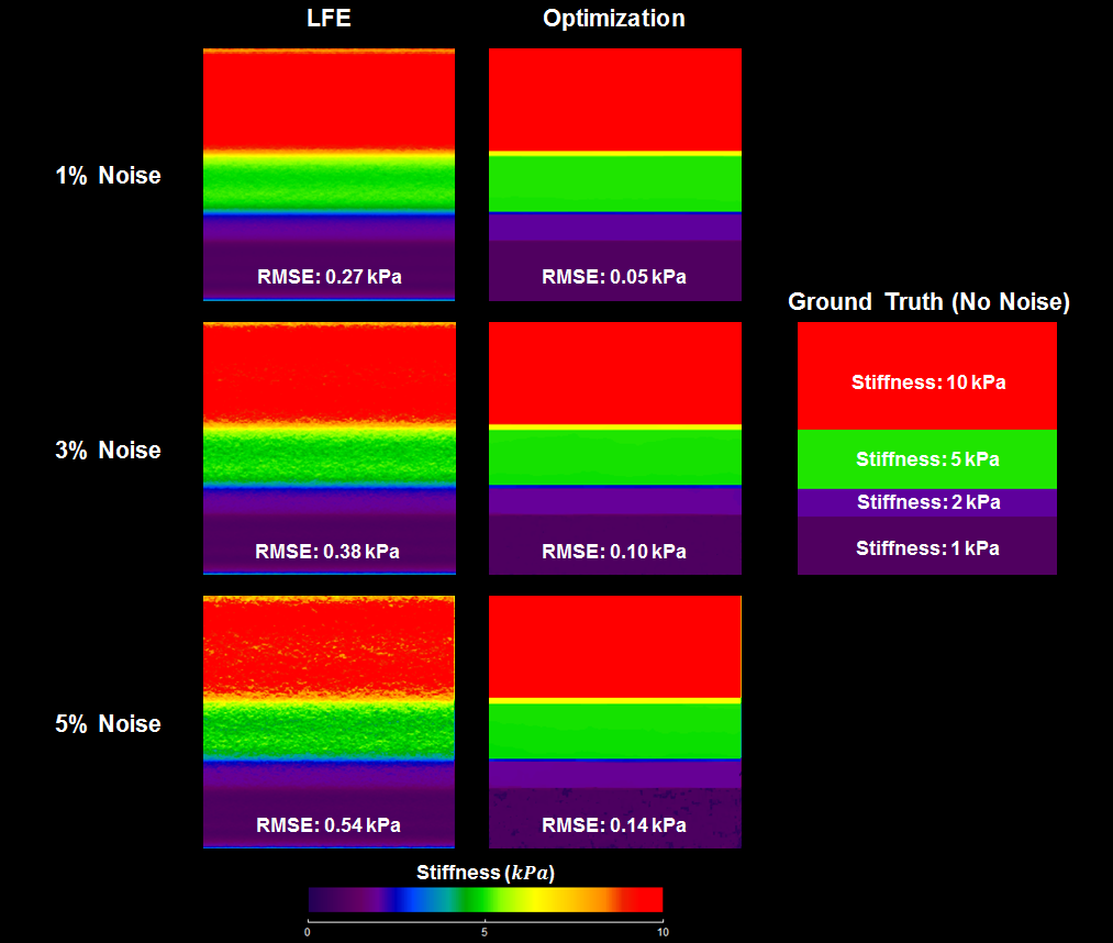
The optimization method yielded lower RMSE and more accurate stiffness maps in simulated phantom when compared to LFE. Figure 1 shows the stiffness maps obtained from both methods. Relatively noiseless stiffness maps were consistently observed in optimization-derived results. The RMSEs of LFE were 0.27, 0.38 and 0.54kPa for 1%, 3% and 5% noise, respectively. The RMSEs of optimization were 0.05, 0.10 and 0.14kPa for 1%, 3% and 5% noise, respectively.
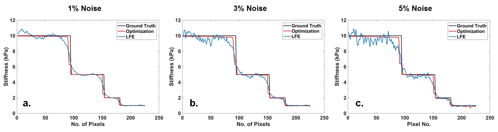
Sharp stiffness transitions were preserved using optimization inversion. Figure 2 displays the line profiles drawn from top to bottom at the center of the ground truth of the simulated data , the optimization-derived and LFE-derived stiffness maps. LFE failed to maintain the sharp transition between different bands due to the well-known edge effect [2]. It was challenging for LFE to distinguish the 2kPa band because of its small width and blurring effect.
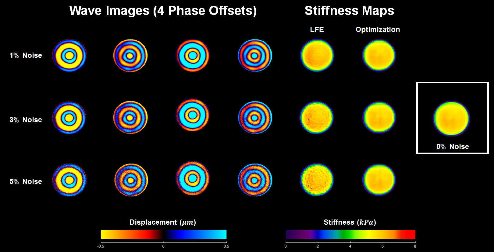
The optimization method was less affected by the presence of noise in the physical phantom data when compared to LFE. Figure 3 demonstrates noisy wave images and stiffness maps obtained using both methods. More consistent and less noisy stiffness estimation was observed in optimization-derived results when compared to LFE-derived stiffness maps.
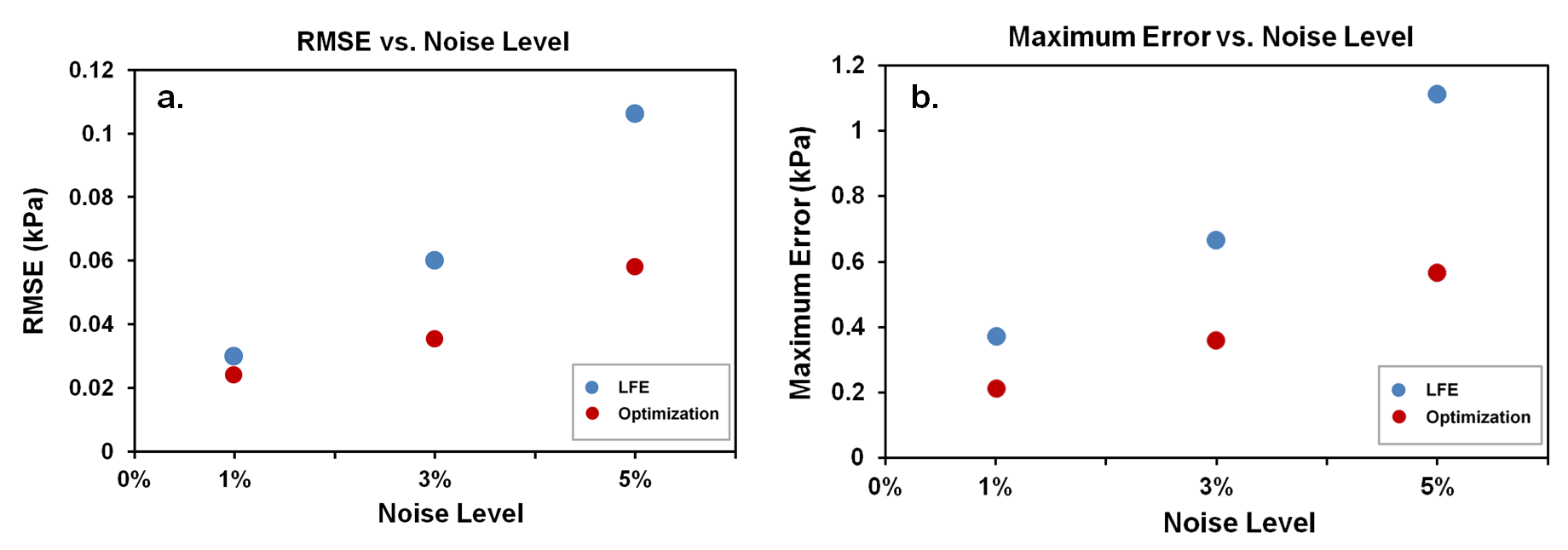
The optimization method yielded lower RMSE and lower maximum error when compared to LFE technique in the physical phantom data. Figure 4 displays the quantitative comparison of both methods.
Conclusion
In this study, the proposed optimization technique yielded stiffness estimation with lower RMSE and lower maximum error when compared to LFE, demonstrating that the optimization technique is able to outperform LFE in the presence of noise.Acknowledgements
No acknowledgement found.References
[1] Muthupillai R, Lomas D, Rossman P, Greenleaf JF. Magnetic resonance elastography by direct visualization of propagating acoustic strain waves. Science 1995;269(5232):1854-1856.
[2] Manduca A, Oliphant TE, Dresner M, Mahowald J, Kruse SA, Amromin E, Felmlee JP, Greenleaf JF, Ehman RL. Magnetic resonance elastography: Non-invasive mapping of tissue elasticity. Med Image Anal 2001;5(4):237-254.
[3] Kruse SA, Smith JA, Lawrence AJ, Dresner MA, Manduca A, Greenleaf, JF and Ehman RL. Tissue characterization using magnetic resonance elastography: preliminary results. Physics in medicine and biology 2000;45(6):1579-1590.
[4] Papazoglou S, Hamhaber U, Braun J, and Sack I. Algebraic Helmholtz inversion in planar magnetic resonance elastography. Physics in medicine and biology 2008;53(12):3147-3158.
[5] Oliphant TE, Manduca A, Ehman RL, and Greenleaf JF. Complex‐valued stiffness reconstruction for magnetic resonance elastography by algebraic inversion of the differential equation. Magnetic resonance in Medicine 2001;45(2): 299-310.
[6] Ting ST, Ahmad R, Jin N, Craft J, Serafim da Silveira J, Xue H, Simonetti OP. Fast implementation for compressive recovery of highly accelerated cardiac cine MRI using the balanced sparse model. Magnetic Resonance in Medicine 2017;77(4):1505-1515.
[7] Paige CC and Saunders MA, LSQR: An Algorithm for Sparse Linear Equations And Sparse Least Squares, ACM Trans. Math. Soft. 1982;8:43-71.
Figures