5520

Whole Brain Absolute CBF Measurements Using Ultra-Low GBCA DCE-MRI and Microsphere Model

Ka-Loh Li¹, Daniel Lewis^1,2, Alan Jackson¹, Sha Zhao¹, and Xiaoping Zhu¹

¹Division of Informatics, Imaging and Data Science, The University of Manchester, Manchester, United Kingdom, ²Department of Neurosurgery, Salford Royal NHS Foundation Trust, Manchester, United Kingdom

Synopsis

Previous authors have attempted to utilize the microsphere model and a maximum gradient (MG) based approach to estimate cerebral blood flow from DCE MRI data, which, however, was not widely accepted. This study developed a new methodology based on the microsphere theory and “early time points” method for mapping absolute CBF, using ultra-low contrast agent dose T1W-DCE-MRI. The new method was assessed using both computer simulation and in vivo data analysis in a patient with GBM, demonstrating that the new method performed better than previous approaches, e.g. MG-based methods, while using much lower dose than perfusion methods based on DSC-MRI.

Introduction

The aim of the study is to develop and assess a new methodology, which is based on the microsphere theory¹ and the “early time points” method (ET)², for absolute CBF estimation using ultra-low dose (1/5 of standard) T1W DCE MRI. Using both Monte Carlo simulation and in vivo study in a patient with glioblastoma multiforme (GBM), we aim to test two specific hypotheses. Firstly, with the low dose compact bolus, the whole upslope segment prior to the first pass peak of the tissue concentration-time curves can be taken as the ET window. Secondly, when the effects of noise are considerable, an averaged concentration (AC) based method, especially when applied on data points located in a segment with higher ENR, is superior to a maximum gradient (MG) based method.

Methods

Patient: The patient with GBM was imaged on a 3.0T Philips scanner. The imaging protocol includes 1) A low dose high-temporal resolution (LDHT) DCE MRI: ∆t = 1.0 s; 3 ml (~0.02 mmol/kg) of contrast agent (CA) administered by power injector at a rate of 3 ml/s, followed by a chaser administered at the same rate. 2) A DSC series, using a 3D PRESTO³.

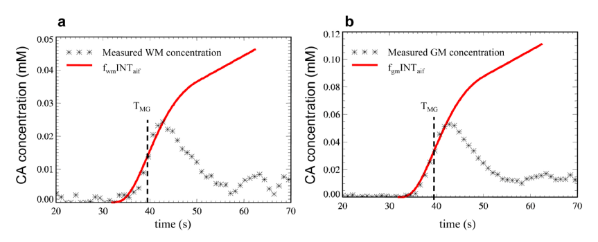
Microsphere model: In DCE MRI, the contrast agent can behave like a microsphere during ‘early time points window (ETW)’, in that no indicator that has arrived in an organ will have yet left it. The microsphere model can be therefore applied:

$$$C_{t}(t)=f\int_{0}^{t} C_{b}(t')dt'$$$ with t ϵ ETW, [1]

where the tissue CA concentration, C_t(t), is equal to the amount of CA delivered to 1 ml of tissue by time t, f is the perfusion term¹ and C_b(t) is the arterial blood concentration. The MG method is then expressed as:

$$$ f=max(\frac{dC_t(t)}{dt})/max(C_{b}(t))$$$ [2]

Assessing the validity of the low dose T1W-DCE MRI data for using the microsphere model: Figures 1a and 1b demonstrate the assessment of whether Eq. 1 holds true for the DCE data from the patient with GBM.

CBF measurement: Five ways for absolute CBF evaluation were compared:

1) The classical MG (MGclassical) method by searching the greatest difference in tissue enhancement between two consecutive data points (i and i+1) on the rising bolus time course.

2) The slope method - The slope over the four points, [i-1, i, i+1, i+2] is used as the numerator in Eq. [2].

3) Averaged concentration referencing t_MG (the ACrMG method), where t_MG = (t_i + t_i+1)/2. The running average of three data points [i+1, i+2, i+3] was used as the value of C_t(t) in Eq. [1].

4) Averaged concentration referencing t_p_eak (the ACrPK method), where t_peak was the tissue peak time. The running average of three data points [i_peak-1, i_peak-2, i_peak-3] was used as the value of C_t(t) in Eq. [1]. For both ACrMG and ACrPK, t = t_MG + 1.5(Δt) = t_{AIF_peak} + 1.5(Δt) was used as the upper time limit in integration of C_b(t).

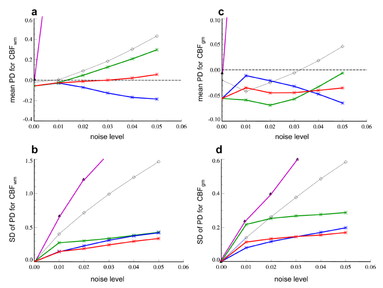
5) Based on the results from Monte Carlo error analysis of the above four methods (Fig. 3), we developed a new method, which takes the average of the CBF values obtained from the ACrMG and ACrPK methods, the ACcomb method.

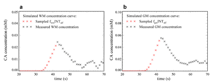
Monte Carlo simulation: Figures 2a and 2b show a simulation of the tissue concentration curves based on the microsphere model. Rician white noise with noise level (= standard deviation/ mean baseline signal) of 1%, 2%, 3%, 4% and 5% respectively was added to the simulated SI-time curves⁴. Absolute CBF values were calculated using the synthetic data sets to produce the so-called ‘measured’ values with the five estimation methods respectively. Percent deviations (PD) of the ‘measured’ values from the ‘true’ values were calculated as: PD = (measured – true)/true∙100%. 20000 repetitions were performed for each method to produce mean and standard deviation (SD) of PD for each CBF estimates.

Results

Figure 3 compares percent deviation in CBF_WM and CBF_GM derived from the five T1W-CBF methods, at various noise levels.

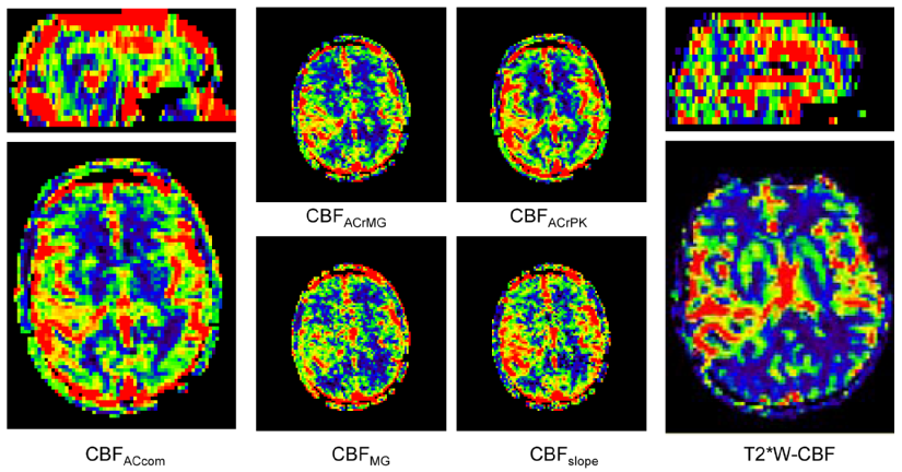
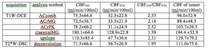
Figure 4 shows the CBF images derived using the T1W_ET methods and the DSC-deconvolution from the patient with GBM. The ROI mean CBF values of the GM, WM and tumor derived from various methods are listed in Table 1.

Both Monte Carlo simulation and in vivo study demonstrated that the AC methods performed better than upslope or MG methods.

Conclusion

The new method is able to provide reliable CBF values using a ultra-low dose DCE MRI acquisition. The ability to provide whole brain 3D coverage with a short acquisition time and low contrast agent dose makes this new method a promising technique for CBF measurement in clinical practice.

Acknowledgements

This work was supported by CRUK [C8742/A18097]. This is a contribution from the Cancer Imaging Centre in Cambridge & Manchester, which is funded by the EPSRC and Cancer Research UK.

References

1. Peters AM. Fundamentals of tracer kinetics for radiologists. Br J Radiol 1998;71(851):1116-1129.

2.. Kwong KK, Chesler DA. Early time points perfusion imaging: theoretical analysis of correction factors for relative cerebral blood flow estimation given local arterial input function. Neuroimage 2011;57(1):182-189.

3. Moonen C, Liu G, Van Gelderen P, Sobering G. A fast gradient-recalled MRI technique with increased sensitivity to dynamic susceptibility effects. Mag Res Med 1992;26:184-189.

4. Li KL, Zhu X, Zhao S, Jackson A. Blood-brain barrier permeability of normal-appearing white matter in patients with vestibular schwannoma: A new hybrid approach for analysis of T1 -W DCE-MRI. J Magn Reson Imaging 2017;46(1):79-93.

Figures

Figure 1. The integrated input curve (INT_aif) was made by integration of the gamma variant fit of the C_b(t); the measured WM and GM curves were averaged concentration-time curves from the whole-volume ROIs. Fig. 1a shows the INT_aif, multiplied by f_wm = 25 ml/min/100ml, and time-shifted to align with the rising bolus time course of the WM concentration curve. Fig. 1b shows the INT_aif, multiplied by f_gm = 60 ml/min/100ml, and time-shifted to align with the rising bolus time course of the GM concentration curve.

Figure 2. Simulation of the ‘theoretical’ tissue concentration curves for Monte Carlo error analysis. Figures 2a and 2b showed the simulated WM and GM concentration curves respectively. The flow-scaled INT_aif and ROI-averaged WM and GM concentration curves used in the simulation were the same as in Figs. 1a and 1b. The upslope part of the theoretical tissue curve was sampled from the flow-scaled INT_aif, while keeping the downslope part, starting from and including the tissue peak time point, of the measured tissue curve.

Figure 3. Mean (3a and 3c) and SD (3b and 3d) of percent deviations for CBF_WM (3a and 3b) and CBF_GM (3c and 3d). For noise levels ≥ 2%, the CBF_WM estimates obtained from the ACrMG and the ACrPK behaved oppositely. The ACcomb estimates CBF_WM with higher accuracy and precision. The CBF_GM estimates showed much less variation in the three averaged-concentration methods, which may be due to the more than twofold greater ENR in the GM uptake curves relative to the WM curves. The ACcomb performed better at a noise level ≥ 4%, but consistently underestimated CBF_GM by about 5%.

Figure 4. The left three columns show CBF images calculated with the five T1W-ET methods. The axial and sagittal view of the 3D CBF_ACcomb were shown on the left column. The right column shows 3D CBF from DSC MRI with a deconvolution method. A comprehensive spatial alignment of the T2*W DSC-MRI to their T1W counterparts permitted effective direct comparison between the maps of T2*W-CBF and T1W-CBF_ET, revealing the expected differences in appearances of the vasculature within both the ‘normal’ brain and the tumor itself due to the susceptibility effects of intravascular contrast in T2*W images

Table 1. ROI mean values of CBF measured from the patient with GBM using different CBF calculation methods, demonstrate that 1) AC methods provide more accurate estimation of in vivo CBF values than classical MG or upslope methods. 2) The mean values of the T2*W-CBF and those of T1W-CBF_ET derived by the AC-based methods for both GM and WM are globally compatible.

Proc. Intl. Soc. Mag. Reson. Med. 26 (2018)

5520