5517
Comparison of arterial input functions measured from dynamic contrast enhanced MRI and computed tomography in prostate cancer patients1Radiology, University of Chicago, Chicago, IL, United States
Synopsis
Arterial input functions (AIFs) measured from dynamic contrast enhanced (DCE) MRI following low dose (0.015 mmol/kg) contrast media were compared with AIFs from DCE CT as ‘gold standard’. Twenty prostate cancer patients received CT and MRI scans on the same day. To correct for different temporal resolution and sampling periods, an empirical mathematical model was used to fit the AIFs and calculate numerical AIFs. Convolution was performed to correct for differences in CT and MRI injection times (~1.5s vs. 30s). MRI and CT AIFs were very similar. Therefore, AIFs can be accurately measured by MRI following low dose contrast agent injection.
INTRODUCTION
Quantitative analysis of dynamic contrast enhanced (DCE) MRI can be achieved by using a pharmacokinetic model. To extract reliable physiological parameters, an accurate arterial input function (AIF) must be measured for each patient1-2. Unfortunately, there is potential for significant error in AIF measurements due to partial volume effects, respiratory motions, inflow artifacts, dose-dependent T2* and water exchange effects3. Here we evaluated the accuracy of AIFs measured from MRI based on AIFs measured from DCE-CT as gold standard. DCE-MRI data were acquired with a low dose (0.015 mmol/kg) of contrast agent. The AIF was measured from prostate cancer patients’ iliac artery. An empirical mathematical model (EMM) was used to fit the AIFs and calculate numerical AIFs (AIFCT and AIFMRI) with matching temporal resolution and sampling period. Then AIFMRI was convolved with a ‘contrast agent injection’ function to correct for differences in the duration of the MRI and CT injections. This allowed quantitative comparison with the AIF measured from CT.METHODS
This study was approved by the Institutional Review Board and informed consent was obtained from all patients. Twenty prostate cancer patients (58±7 years) were enrolled in this study. DCE-CT scans (120mL Omnipaque350 was injected at 4mL/s with duration of 30 s) were performed on a Philips Brilliance iCT scanner at 120 kVp with 29 dynamics, a temporal resolution of 5s for the first 25 dynamics followed by 2 dynamic scans 1 min apart and, subsequently, 2 dynamics scans 2 min apart. The default scan length was 8 cm with a 128×0.625 mm beam configuration. The DCE-CT temporal resolution and number of scans was limited due to radiation dose considerations and contrast agent volume. The MRI scan was performed ~3 hours after the CT scan on a Philips 3T scanner. After other clinically required scans, variable flip angle (VFA) 3D-FFE-T1 sequences were acquired. Subsequently, 90 ultra-fast DCE-MRI scans were acquired using an mDixon sequence (TE1/TE2/TR=1.5/2.8/4.2 ms, FA=10°, FOV=18×37×8cm3, in-plane resolution=1.5×2.8×3.5mm3, temporal resolution=1.5 s). A low dose (0.015 mmol/kg) of Gadolinium-based contrast agent was injected in ~1.5 s. AIFs were extracted from the iliac arteries. AIF Iodine and Gd concentrations were corrected for the total injected dose (mM/dose). Due to differing temporal resolutions, contrast agent injection durations, and duration of following contrast agent, the AIFs obtained from CT and MRI could not be directly compared. An empirical mathematical model (EMM) was employed to fit the AIFs:
$$AIF(t)=tan^{-1}(t/30)\cdot[1+\sum_{n=1}^2A_{n}exp(-(t-\tau_{n})^{2}/2\sigma_{n}^{2})]\cdot B\cdot exp(-\beta\cdot t)$$
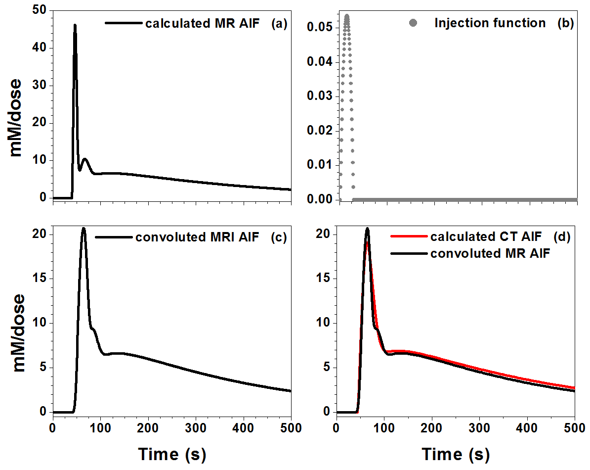
where An and B are scaling constants, $$$\tau_{n}$$$ and σn (n=1,2) are the center and width of a Gaussian function, and β is the decay constant. The resulting EMM’s were used to calculate CT AIF (AIFCT) and MRI AIF (AIFMRI) at temporal resolution of 0.5 s, ending at 8.3 minutes. The AIFMRI was further corrected for the difference in injection times between CT and MR (1.5 s vs. 30 s) by using convolution:
$$AIF_{MRI}^{con}(t)=AIF_{MRI}(t)\otimes\ h(t)$$
where $$h(t)=\frac{M-(t-t_{0})^{2}}{A}$$ is the injection function ( M=196.0,
A=3658.66, t=0 to 28.5 s, t0=14.25 s). The parameters M
and A were determined so that integral
of h(t) is 1 and its width is 28.5 s.
RESULTS
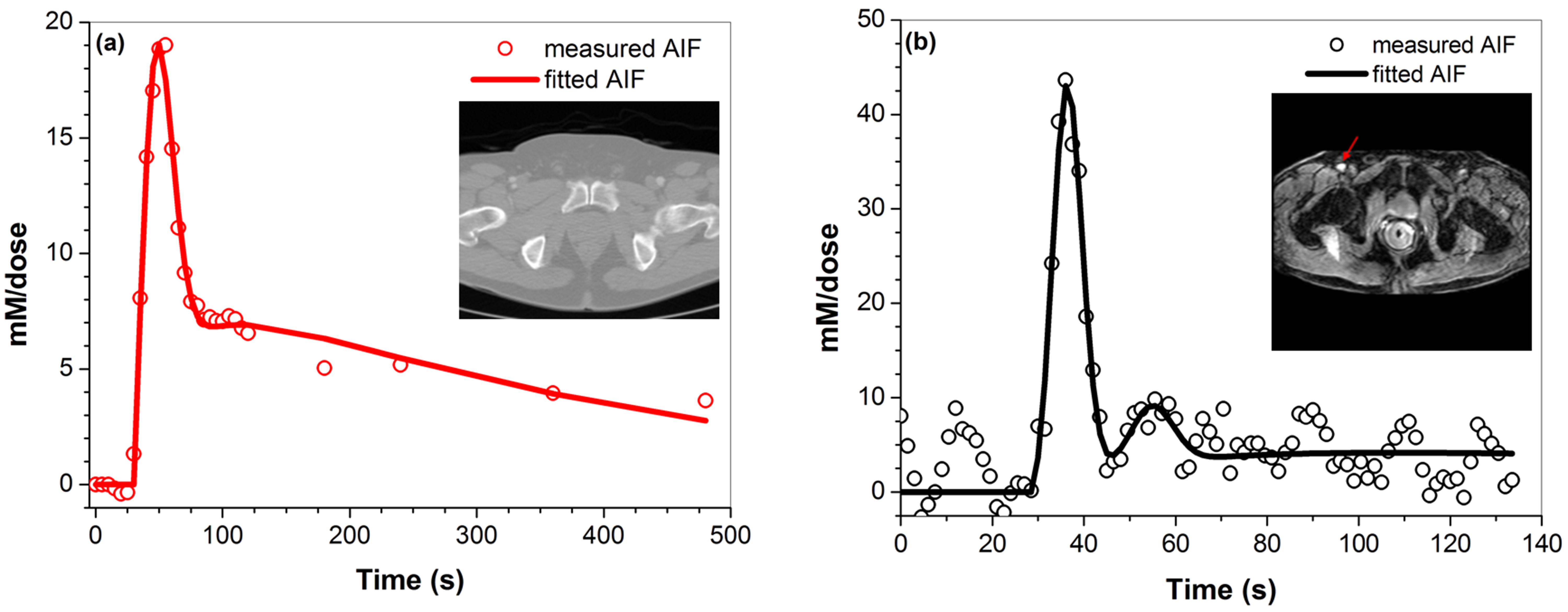
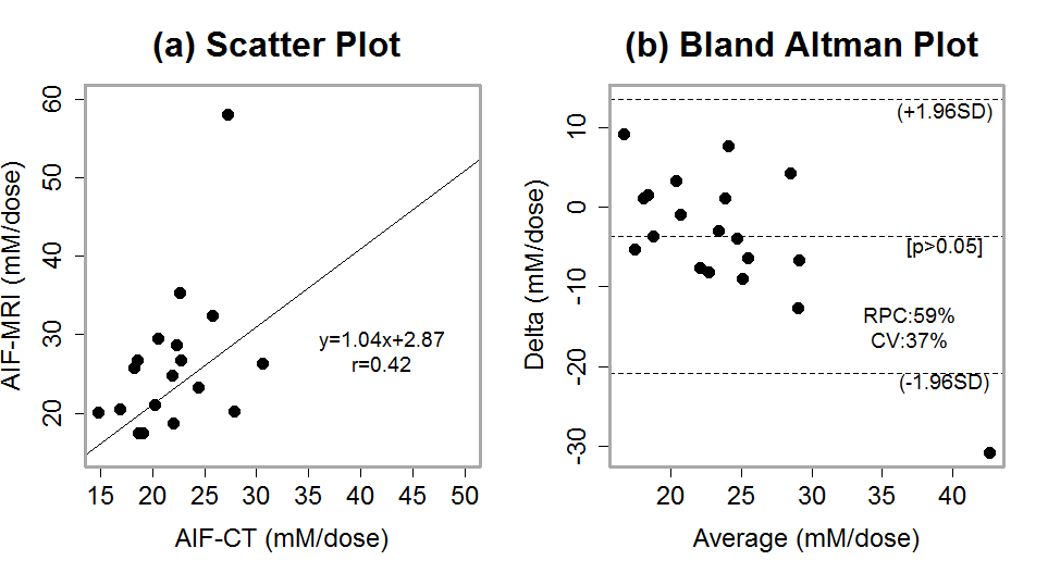
Figure 1 shows a typical AIF measured from: (a) CT and fitted with the EMM, and (b) MRI and fitted with the EMM for the same patient. Figure 2 shows the MRI AIF calculated with high temporal resolution and convoluted with injection function: (a) numerical AIFMRI, (b) injection function h(t), (c) convoluted AIFMRIcon, and (d) overlays numerical AIFCT and AIFMRIcon. The average goodness-of-fit value R2 between AIFCT and AIFMRICON was 0.74±0.20, indicating good agreement. The full width at half maxima of AIFCT and AIFMRI were 30.4±2.4 s and 37.2±15.5 s respectively. There was no significant difference (p>0.05) between the peak amplitude of AIFCT (22.2±4.1 mM/dose) and convoluted AIFMRICON (26.2±9.7 mM/dose). Figure 3 shows (a) correlation of the maximum values of AIFCT and AIFMRICON, and (b) the Bland-Altman plot. The variation from the mean value of measured iodine concentration (17%) is less than the variation from the mean for gadolinium concentrations (48%).DISCUSSION
The EMM was used to fit both CT and MRI AIF, and consequently high temporal resolution AIFs were calculated with the same sampling duration. Convolution was used to correct the AIFs for differences in contrast agent injection duration. The results demonstrate that the AIFs measured directly from the iliac artery by DCE-MRI following a low dose of contrast agent were consistent with the ‘gold standard’ AIFs measured by CT. This indicates that AIFs can be accurately measured by ultra-fast DCE-MRI.Acknowledgements
This research is supported by NIH R01 CA172801-01 and NIH 1S10OD018448-01.References
1. Korporaal, J. G., Van Den Berg, C. A., Van Osch, M. J., Groenendaal, G., Van Vulpen, M. & Van Der Heide, U. A. 2011. Phase-based arterial input function measurements in the femoral arteries for quantification of dynamic contrast-enhanced (DCE) MRI and comparison with DCE-CT. Magn Reson Med, 66, 1267-74.
2. 1. Wang, H. & Cao, Y. 2012. Correction of arterial input function in dynamic contrast-enhanced MRI of the liver. J Magn Reson Imaging, 36, 411-21.
3.
Parker, G. J., Roberts, C., Macdonald, A., Buonaccorsi, G. A., Cheung, S.,
Buckley, D. L., Jackson, A., Watson, Y., Davies, K. & Jayson, G. C. 2006.
Experimentally-derived functional form for a population-averaged
high-temporal-resolution arterial input function for dynamic contrast-enhanced
MRI. Magn Reson Med, 56, 993-1000.
Figures