5516
Robust SNR determination based on Resampling for Quality Control and Workflow Support in Quantitative DCE perfusionJakob Meineke1, Karsten Sommer1, and Jochen Keupp1
1Philips Research Europe, Hamburg, Germany
Synopsis
A Monte-Carlo method is used to compute and predict SNR of image data for quantitative DCE-MRI perfusion measurements. This information can be used for quality assurance and to improve imaging workflow.
Introduction
The accurate quantification of SNR is important for quantitative MRI and quality control in general1. This is particularly true for modalities working in the low SNR limit due to the need for high spatio-temporal resolution, such as DCE-MRI for quantitative perfusion and permeability measurements. For example, a precise knowledge of SNR enables the determination of expected statistical errors for native tissue T1-mapping and contrast-agent (CA) concentration determination. A real-time estimate of SNR would allow to adjust the imaging sequence before contrast-agent injection and avoid sub-standard scans, which cannot be used for robust quantitative analysis. Nevertheless, efforts to quantify SNR rarely go beyond the “two-region” method2, which is known to be wrong when multi-channel receiver arrays, parallel imaging, and other modern MRI methods are employed. To overcome this limitation, a Monte-Carlo based method, similar to Robson et al.3, is applied in this work, which is based on resampling noise-calibration data for determining and predicting SNR in DCE-MRI exams.Background
Two important parts of a DCE-MRI exam are T1-mapping based on the Variable Flip-Angle (VFA) method, followed by a dynamic scan (DCE scan) during CA injection. To predict the SNR of the dynamic scan, the SNR is first determined from at least one of the VFA scans using the method described below. Applying a suitable signal model, the obtained signal for any of the VFA scans can be scaled to predict the expected signal of the DCE scan. Here, for simplicity, the Ernst equation is employed, which describes the signal of fully transverse spoiled gradient-echo sequences. The same noise calibration measurement can be used to generate noise images of the dynamic scan even before the scan is started, thus leaving time for intervention. Creation of noise images: Given a set of samples $$$s_j$$$, representing complex noise measured for the j-th element of a multi-channel receive array with N channels, the noise covariance matrix C is defined as $$$C_{ij}=<s_i^* s_j>$$$. Following diagonalization, $$$C=UDU^{H}$$$, a single noise sample is computed by drawing from N independent, complex Gaussian random variables $$$\rho_k$$$, to compute $$$s_i=U_{ij} \sqrt{D_{jk}}\rho_k$$$. The k-space of the sequence of interest is filled with noise samples, and reconstruction proceeds as usual, this including effects of coil-combination, filtering, etc. The statistical noise distribution can be determined on a voxel-by-voxel basis from a suitable number of individual noise realizations, allowing the estimation of pure noise image4.Methods
T1-weighted
gradient echo scans (FOV: 216×216×95 mm3, acquisition voxel: 1.5×1.5×5 mm3, TE/TR:
2.5/7 ms, 10 dynamics) with different flip-angles (2,5,10,20,30) were acquired
for a gel phantom with 12 tubes of varying T1 and T2 values (Diagnostic Sonar,
Livingston, UK) using 13-ch head coil at 1.5T (Ingenia, Philips, Best, The
Netherlands). The noise resampling was implemented as a new node within the scanner
manufacturer’s reconstruction software
framework (Recon 2.0). Noise
images were generated computing the standard-deviation across the stack of resampled
noise images and for the acquired dynamics.
From the scans with flip-angles from 2°-20°, a T1-map was created using the
variable-flip angle method (VFA)5. Based on the Ernst equation, $$$S(\alpha, T_1, T_R)=M_0\sin(\alpha)\frac{1-\exp(-T_R/T_1)}{1-\cos(\alpha)\exp(-T_R/T_1)}$$$,
assuming M0=1, and the T1-map, the mean
magnitude signal of the scan with flip-angle 30° was predicted by scaling the signals obtained from the other
scans. Finally, directly determined SNR and predicted SNR were compared within
ROIs defined within the tubes of the phantom, and sorted according to the
determined T1 values.Results
Figure 1 shows obtained SNR maps computed from pure noise images obtained via resampling and by using the direct method. Tubes with short T1 show high SNR. Also clearly visible is the variation in SNR across the field-of-view due to the spatially varying noise level. The spatial variation of the noise level, also presented directly in Figure 2, reflects the variation of coil-sensitivities but also from parallel imaging. Figure 3 demonstrates the excellent agreement between the directly measured SNR of the scan with flip-angle 30° and the SNR predicted from the scan at 5°.Discussion and Conclusion
Noise-level maps determined using a Monte-Carlo method were used to predict SNR of a different scan with high accuracy over a large range of T1 values. This prediction is useful for quality assurance and workflow support, for example, for quantitative DCE-MRI, where scans cannot be repeated once the CA is injected. The presented method requires no additional measurements and generalizes to different acquisition and reconstruction methods. The method allows the reliable determination of an upper bound across the imaged region and characterization of spatial noise-correlations. Furthermore, the noise-level maps obtained using the resampling method in combination with the direct method applied to dynamic scans, could be used to determine quality criteria for motion compensation techniques or image registration.Acknowledgements
No acknowledgement found.References
- Gedamu et al, JMRI 28, 308 (2008)
- Kaufman et al, Radiology 173, 265 (1989)
- Robson et al, MRM 60, 859 (2008)
- National Electrical Manufacturers Association (NEMA). NEMA Standards Publication MS 1-2001. Rosslyn: National Electrical Manufacturers Association; 2001. 15 p.
- Helms et al., Identification of signal bias in the variable flip angle method by linear display of the algebraic Ernst equation, MRM 66, 669 (2011)
Figures
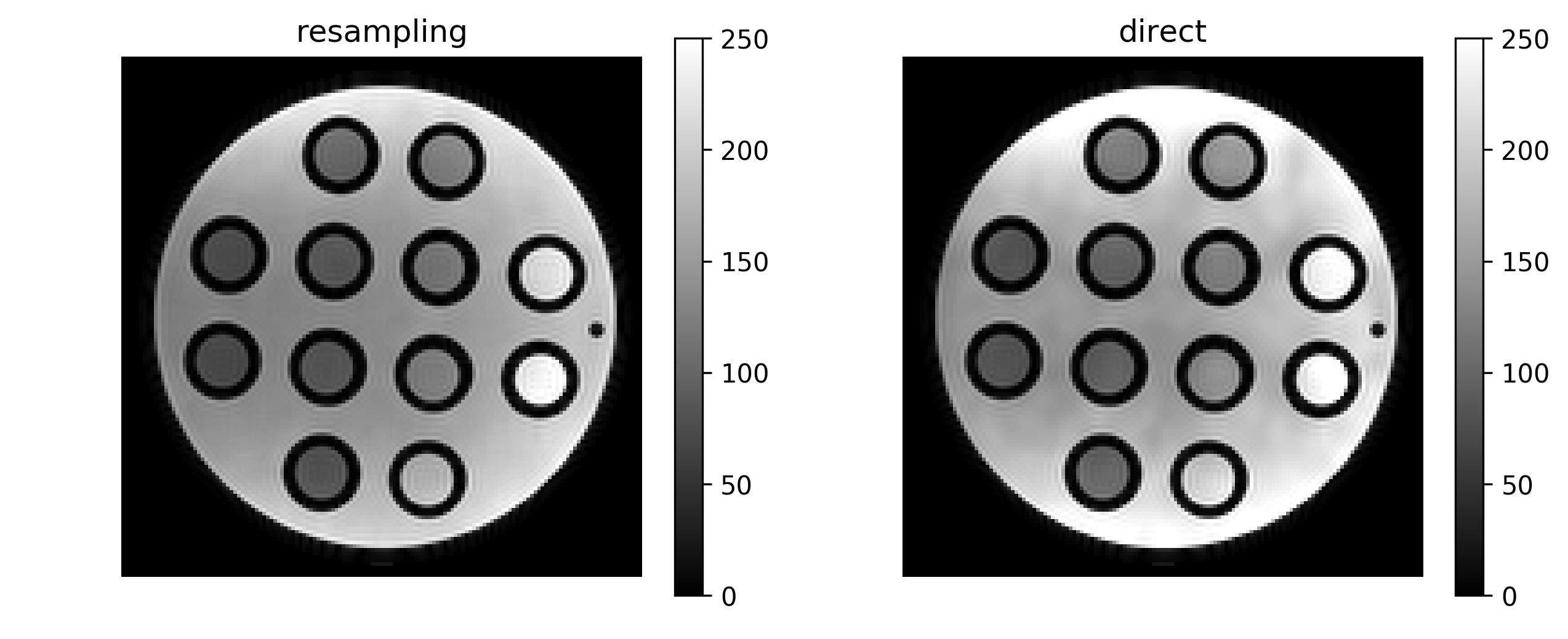
Figure 1: Example SNR
maps obtained using resampling method (left) and direct method (right) for the
scan at flip-angle 10°.
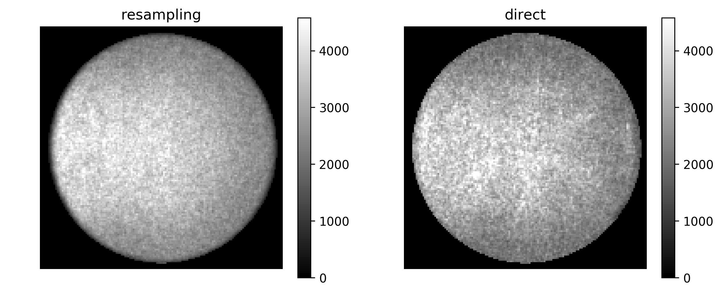
Figure 2: Example noise
level maps obtained using resampling method (left) and direct method (right).
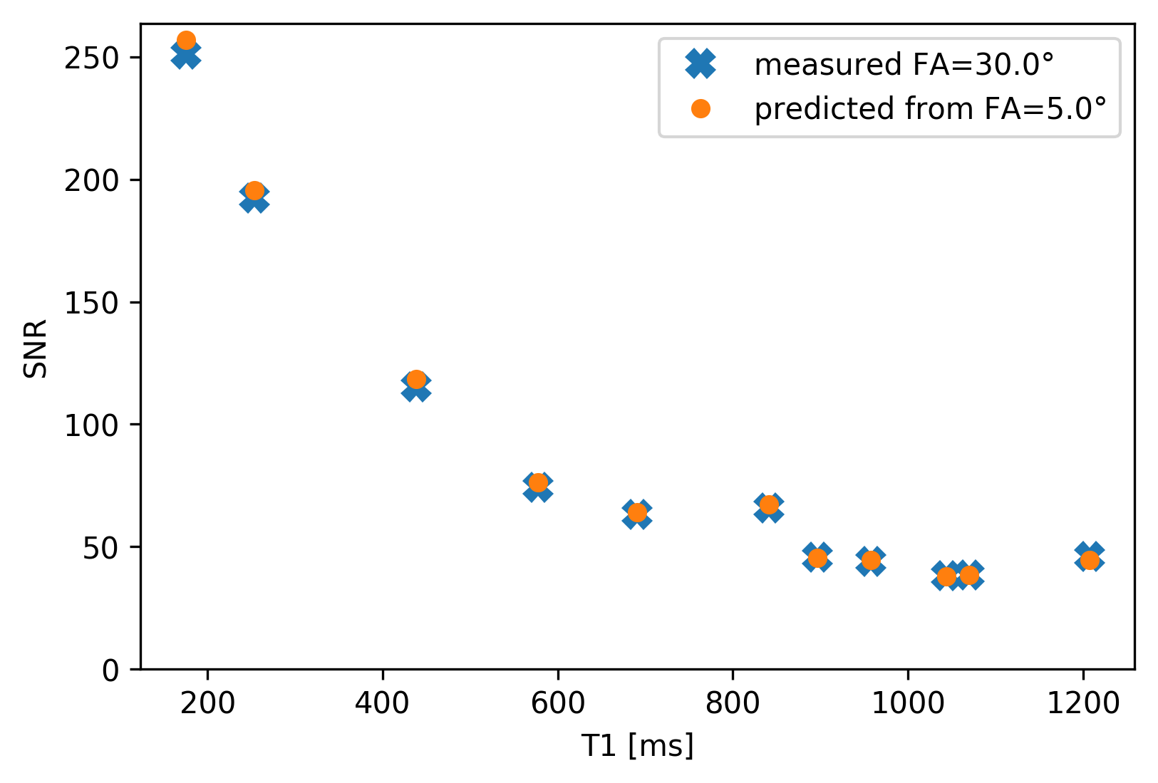
Figure 3: Comparison
of predicted SNR and directly measured SNR as a function of T1 in the tubes of
the phantom. SNR was predicted by scaling the signal from the measurement at
flip-angle 5° using the RF-spoiled signal model and using the resampling method
to generate the noise level image. The measured SNR for the scan at flip-angle
30° was computed using the direct method, i.e. using mean and standard-deviation
across dynamics.