5482

Frequency Characteristics of Blind-Deconvolved Resting-State Networks using Empirical Mode Decomposition

Dietmar Cordes^1,2, Muhammad Kaleem³, Xiaowei Zhuang¹, Karthik Sreenivasan¹, Zhengshi Yang¹, Tim Curran², and Virendra Mishra¹

¹Cleveland Clinic Lou Ruvo Center for Brain Health, Las Vegas, NV, United States, ²University of Colorado, Boulder, CO, United States, ³University of Management & Technology, Lahore, Pakistan

Synopsis

Energy-period relationships and frequency content of Intrinsic Mode Functions (IMFs) were studied in deconvolved fMRI data using a blind deconvolution method. Results are shown for multiband MB8 resting-state data collected with a TR of 0.765s for a group of 22 healthy subjects. Findings of the present study suggest that high-frequency content in the major primary resting-state networks (such as the Default Mode Network, Visual Network, Auditory Network, or Fronto-Parietal network) is rather limited and not supported to be of any significance for high frequencies larger than 0.21 Hz, whether in BOLD data or blind-deconvolved data.

Introduction

Resting-state functional networks were traditionally computed by low-pass-filtering data retaining frequencies less than 0.1Hz¹. Recently, it was argued that high frequencies larger than 0.1Hz may also contribute to functional connectivity for major resting-state networks^2,3. To shed more light on this question, we applied a blind-deconvolution method to resting-state data that were collected with a high sampling rate, allowing to investigate the frequency content up to 0.65Hz. Rather than relying on user-defined frequency bands, we use Empirical Mode Decomposition (EMD)^4,5 to study the natural occurring frequency bands of major resting-state networks after blind deconvolution and compare results with the original BOLD data.

Methods

FMRI was performed on 22 healthy subjects in a 3T Siemens MRI scanner (32-channel head coil, MB8 EPI, TR 765ms, TE 30ms, flip 44deg, 2380 time frames). The data have been minimally preprocessed to avoid contamination of high-frequency artifacts that could have been potentially introduced by improper preprocessing. Identification of resting-state networks was done by using group ICA. For blind deconvolution we used the method by Wu et al.⁶ Briefly, each fMRI time series was treated as a convolution of point processes with unknown hemodynamic response function (HRF) and delay time. The HRF was approximated by a linear combination of the canonical HRF, its first order and second order derivative. The expansion coefficients were obtained by least square minimization, and the best time delay (for each voxel) was obtained by covariance minimization of the residual. Deconvolution was then carried out using the Wiener filter in the Fourier domain. After deconvolution group ICA (using the FastICA algorithm⁷) was used to obtain 30 spatial components. Using visual inspection, the Default Mode Network (DMN), the primary and secondary visual networks (VIS, VIS2), the auditory network (AUD) and the left/right frontoparietal network (lFPN, rFPN) were identified. The corresponding time courses were computed by spatial regression and then further decomposed into Intrinsic Mode Functions (IMFs) using EMD.

Results

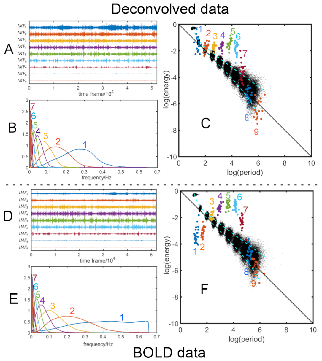
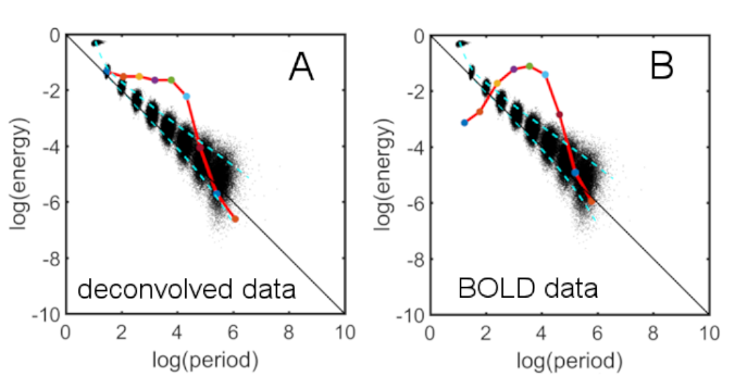
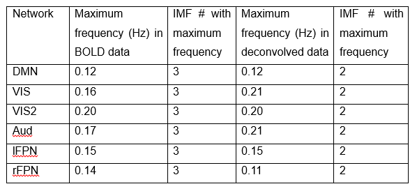
Fig.1 shows time series characteristics of the first 9 IMFs for the DMN after deconvolution (Fig.1A-C). Comparison to the original BOLD data are shown in Fig.1D-F. Note that IMF1 and IMF2 have large amplitudes of oscillation (Fig.1A) compared to the original data (Fig.1D). Furthermore, the frequency range of IMF1 is limited to the intermediate frequencies (Fig.1B), which is quite different than the wide frequency spectrum of IMF1 of the BOLD data (Fig.1E). Fig.1C and Fig.1F show the energy-period relationship of the IMFs superimposed on a white noise spectrum (black dots). Note that the mean energies of IMF1 and IMF2, which represent mostly frrquency components above 0.1Hz, are significantly increased for the deconvolved data. However, the corresponding mean energy-period points do not extend above the white noise spectrum. Fig.2 shows the energy-period signatures averaged over all 6 resting-state networks showing that the deconvolved data (Fig.2A) have an IMF signature that is closer to the white noise distribution when compared to the signature of the BOLD data (Fig2.B). To obtain more frequency-specific information, we also high-pass filtered the IMFs and computed the related spatial maps by regression on the original deconvolved data. Table 1 lists the highest frequency content of each network to achieve a Dice similarity coefficient larger than 0.7.

Discussion

IMFs of deconvolved data are characterized by a lower mean frequency and lower frequency range than corresponding IMFs of BOLD data. From the energy-period plots and Fig.1B vs Fig.1E, it is apparent that the period is increased for all IMFs of the deconvolved data. Attenuation of high frequencies larger than 0.3 Hz can be explained by the Wiener filter to prevent noise amplification. In contrast, the energy of IMF1 and, to a lesser degree, IMF2 are increased compared to the BOLD data. For all other IMFs the energy is relatively similar to the BOLD data. It appears that a large portion of the amplified frequencies by deconvolution is not network associated and only increases the energy density of IMF1 and IMF2, and network-associated frequencies are not shifted to higher frequencies. From the energy-period relationship, it can also be seen that blind deconvolution leads to signatures that are closer to signatures of white noise data.

Conclusion

This study suggests that blind deconvolution amplifies mostly intermediate frequencies (0.2 Hz-0.3 Hz) which are not network-related. Also, high frequencies larger than 0.3 Hz are attenuated by the Wiener filter, and energy-period signatures of IMFs are shifted more towards the diagonal line that is associated with white noise processes. Low frequencies less than 0.1 Hz provide the largest contribution to the studied networks, and none of the primary networks could be associated with any significant frequency content above 0.21 Hz.

Acknowledgements

This research project was supported by the NIH (COBRE grant 1P20GM109025 and 1R01EB014284).

References

[1] Cordes D, et al. Frequencies contributing to functional connectivity in the cerebral cortex in resting-state data. AJNR 2001, 22:1326-1333.

[2] Niazy RK, et al. Spectral characteristics of resting-state networks. Prog. Brain Res. 2011, 193:259-276.

[3] Chen JE, Glover GH. BOLD fractional contribution to resting-state functional connectivity above 0.1Hz. NeuroImage 2014, 107:207-218.

[4] Flandrin P, et al. Empirical mode decomposition as a filter bank, IEEE Sig. Proc. Letters 2004, 11(2), 112-114.

[5] Huang NE, et al. The empirical mode decomposition and the Hilbert spectrum for nonlinear and non-stationary time series analysis. Proc. R. Soc. Lond. 1998, A 454, 903-995.

[6] Wu GR, et al. A blind deconvolution approach to recover effective connectivity brain networks from resting state fMRI data. Medical Image Analysis 2013, 17:365-374.

[7] Hyvärinen A. Fast and Robust Fixed-Point Algorithms for Independent Component Analysis. IEEE Transactions on Neural Networks 1999, 10(3):626-634.

Figures

Fig.1: Deconvolution of the fMRI data and analysis of the DMN by EMD. (A) shows the first 9 IMFs of the DMN. The frequency content of the IMFs are shown in (B). Note that IMF1 has a medium frequency spectrum whereas the higher-order IMFs have a narrow-band low-frequency spectrum. (C) shows the energy-period relationship of the IMFs superimposed on white noise (black dots). Each colored dot represents a subject. Note the increased energy of IMF1 and IMF2. Subplots (D,E,F) show the corresponding information of the original fMRI data without deconvolution. Note that IMF1 and IMF2 have very low energy.

Fig.2: Energy-period feature vectors of the first 9 IMFs for deconvolved data (A) and original BOLD data (B), averaged over major resting-state networks (DMN, VIS, VIS2, AUD, lFPN, rFPN). White noise profiles are indicated by black dots. Note that deconvolved data are closer to the white noise profile and have more energy in the lower index IMFs.

Table 1: Frequency-content of high-pass filtered intrinsic mode functions (IMFs) with significant Dice coefficient (> 0.7) for different resting-state networks. Note that IMFs of deconvolved data lead in general to a smaller peak frequency, FWHM, and frequency range than IMFs of BOLD data. For the DMN, we were not able to find any significant frequency contribution above 0.12Hz. It appears that in general high frequencies above 0.21Hz have negligible contribution to the studied networks.

Proc. Intl. Soc. Mag. Reson. Med. 26 (2018)

5482