5481
Can Sensitivity and Specificity Be Gained Simultaneously in Neuroimaging?1SSCC/DIRP/NIMH, National Institutes of Health, Bethesda, MD, United States, 2University of Maryland, College Park, MD, United States, 3National Institutes of Health, Bethesda, MD, United States
Synopsis
Whole brain analysis currently faces two challenges: the increasing demand of correction for multiplicity and the usual tug of war between specificity and sensitivity. In addition, sensitivity suffers substantially because of stringent correction, while specificity is not directly considered when forming clusters. Specificity can be largely guaranteed through ROI-based analysis if ROIs can be a priori defined. Furthermore, sharing information across ROIs through an integrated model can improve model efficiency and detection power. We offer an alternative or complementary approach to the conventional methods in resolving the dilemma of multiple comparisons and dichotomous decisions. Lastly, through the approach, we promote totality and transparency in results reporting, and avoid the hard thresholding of a p-value funnel.
Introduction: challenges with correction for multiple comparisons, sensitivity and specificity, incorrect sign and magnitude
Many investigators have felt the jolt after the recent discussion1 regarding stringently controlling false positive rate (FPR) due to multiple comparisons. As the data are fitted with as many models as the voxels, correction for multiplicity is required to gain legitimacy in controlling FPR. Regardless of correction methods, cluster size (often combined with signal strength) plays a leveraging role, with a higher threshold leading to a smaller cluster cutoff, therefore a neurologically slender region can only gain ground with a low p-value while large regions with a relatively high p-value may fail to survive the criterion. Similarly, a lower threshold requires a higher cluster threshold, so smaller regions have little chance of meeting the threshold.
We raise the question as to whether controlling FPR under null hypothesis significance testing (NHST) is unnecessarily over-conservative. More fundamentally, we echo the ongoing debate as to whether the adoption of dichotomous decisions is appropriate where the null hypothesis (no effect) is not even pragmatically meaningful. When noise inundates signal, two different types of error2 are more relevant than FPR: incorrect sign (type S) and incorrect magnitude (type M).
Here we introduce an efficient strategy through Bayesian hierarchical modeling (BHM): turning the focus of FPR into quality control by calibrating type S errors while maintaining reasonable statistical power. The efficiency is demonstrated through an application at ROI level which allows all regions on an equal footing by ensuring smaller regions are not disadvantaged simply because of size. In addition, their signal strengths are calibrated among themselves, dissolving multiplicity under one holistic model. Compared to GLM, BHM may achieve increased specificity and sensitivity simultaneously, and its superiority is illustrated in model performance and quality check through a dataset.
Theory: Bayesian hierarchical modeling (BHM)
There is a long history of arguments that emphasize the problems with NHST3. For example, it is vulnerable to misinterpret the conditional probability as the probability of the null event conditional on the data; the difference between a statistically significant effect and an insignificant effect may not necessarily be significant. Moreover, simulations2 have shown that, in low power cases, type S errors can reach 50%. With loss of generality, we model the data at r ROIs from n subjects through r separate GLMs,
$$y_{ij}=a+bx_i+\epsilon_{ij},$$
where i and j code for subject and ROI, y, x, and $$$\epsilon$$$ represent the response data, explanatory variable and residuals, a and b are regression coefficients. With r GLMs, correction for FPR is warranted under NHST, which is why ROI-based analysis is rarely performed except for graphical presentations. However, those ROIs are not isolated entities; instead, they all reveal neurological activities with the same scale and range. Such commonality should be utilized and incorporated into the analytical pipeline. By merging the data, we formulate a BHM,
$$y_{ij}|a_j,x_i,b_j\sim N(a_j+b_jx_i,\sigma^2),i=1,2,...,n;j=1,2,...,r,$$
where $$$a_j$$$, $$$b_j$$$, and $$$\sigma^2$$$ are the intercept and slope effects for each ROI, and residual variance. With Gaussian priors for $$$a_j$$$ and $$$b_j$$$, we perform a full Bayesian analysis, and derive their posterior distributions. With one holistic BHM instead of r separate GLMs, multiplicity is dissolved: the r effects, $$$a_j$$$ or $$$b_j$$$, are calibrated among the r ROIs through shrinkage.
Results: application of BHM to a real dataset
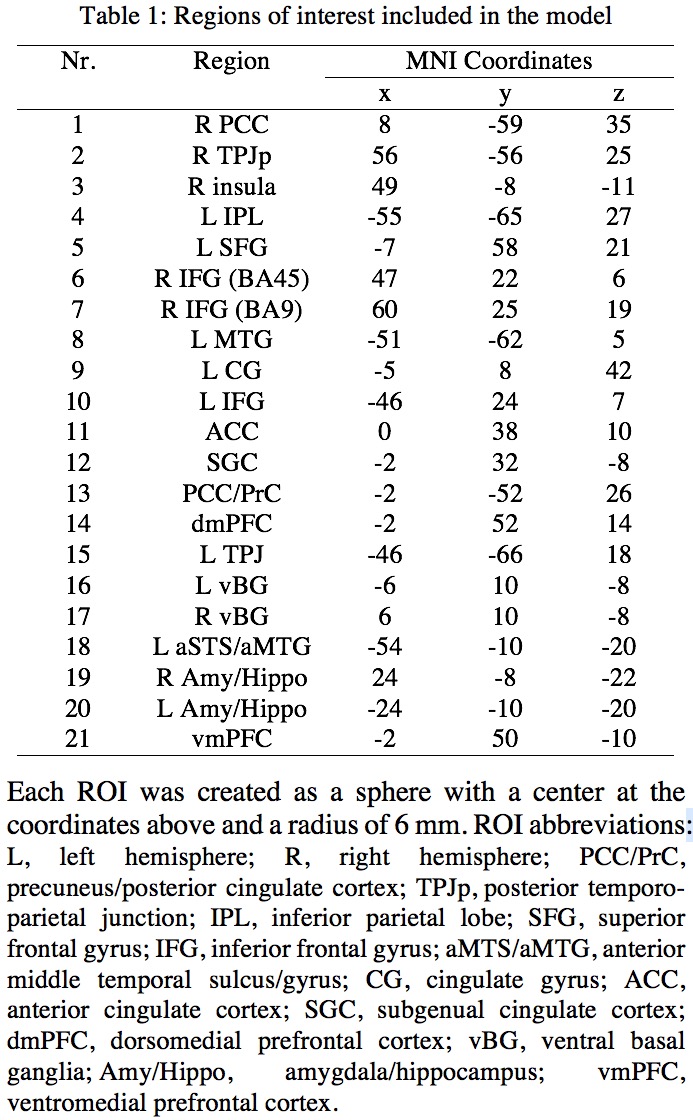
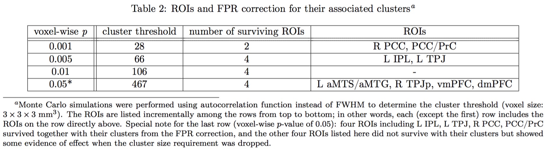
Twenty-one ROIs (Table 1) were selected for their potential relevancy to a resting-state study4, and mean z-scores were extracted at each ROI from the output of seed-based correlation analysis (seed: right temporo-parietal junction) with 124 subjects. The effect of interest at group level is the correlation between a behavioral measure, overall Theory of Mind Inventory, and the association with the seed. Traditional whole brain analysis showed the difficulty with some clusters surviving FPR correction (Table 2).
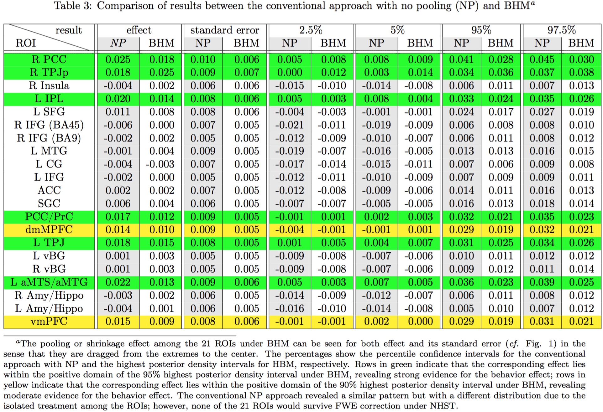
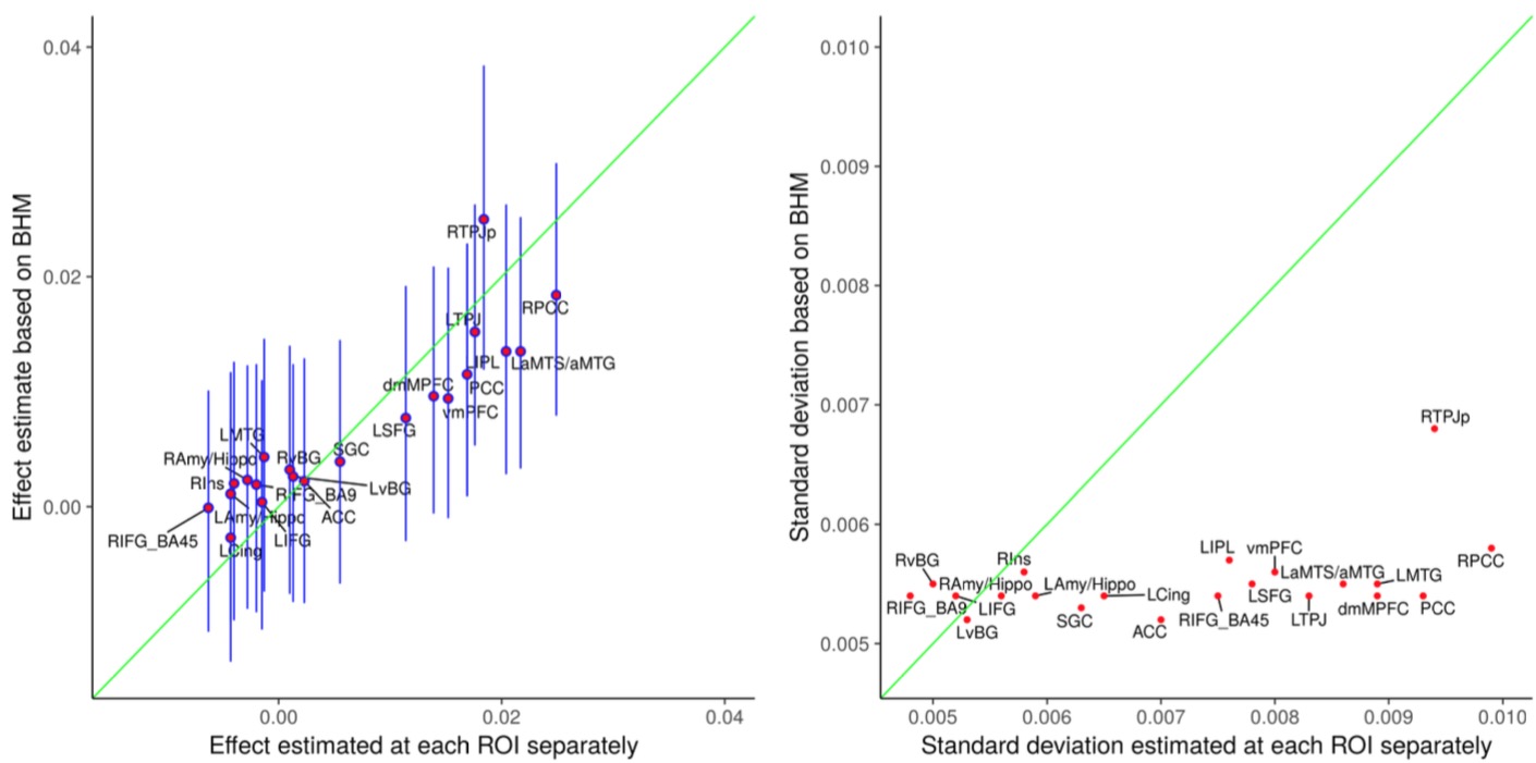
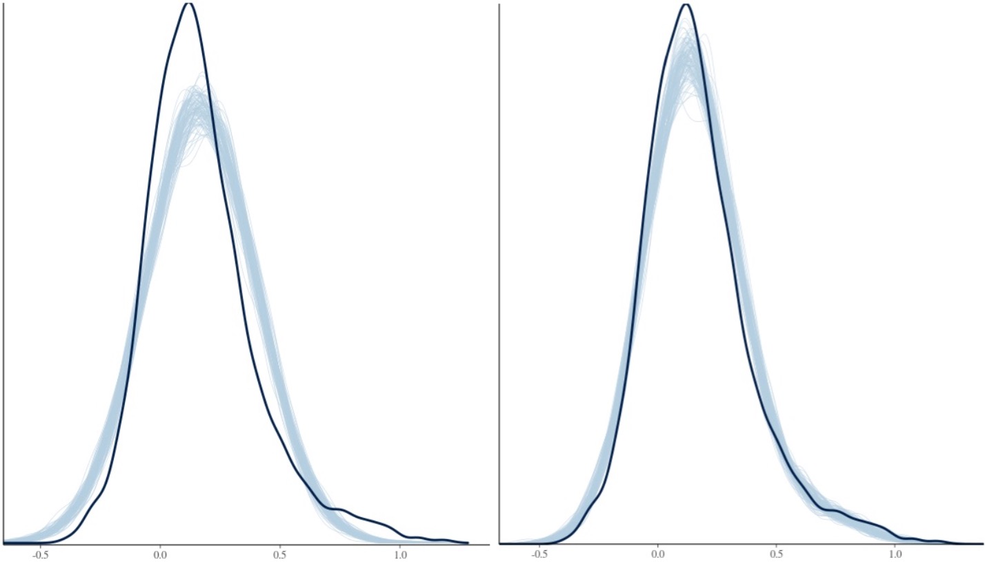
The ROI data were reanalyzed with BHM through Stan5 (Table 3). Compared to traditional GLM, the shrinkage effect under BHM can be seen for both the effect and its standard error (Table 3, Fig. 1). Although GLM renders similar inference among the ROIs, the burden of FPR correction (e.g., Bonferroni) is too severe. More importantly, the quality and fitness of BHM can be verified through posterior predictor check (Fig. 2) that compares the observed data with the simulated data based on the model.
Conclusion: advantages of BHM over GLM
By focusing on an ensemble of predefined ROIs, we demonstrate the advantage of BHM in controlling type S errors and in achieving reasonable sensitivity and specificity. In addition, BHM is well aligned with the recent discussion surrounding the fundamental problems with the conventional statistics paradigm.Acknowledgements
The research and writing of the paper were supported (GC, PAT, and RWC) by the NIMH and NINDS Intramural Research Programs (ZICMH002888) of the NIH/HHS, USA, and by the NIH grant R01HD079518A to TR and ER. Much of the modeling work here was inspired from Andrew Gelman's blog. We are indebted to Paul-Christian Beurkner and Stan development team members Ben Goodrich, Daniel Simpson, Jonah Sol Gabry, Bob Carpenter, and Michael Betancourt for their help and technical support. The figures were generated using ggplot2 in R.References
1Eklund, A., Nichols, T.E., Knutsson, H., 2016. Cluster failure: Why fMRI inferences for spatial extent have inflated false-positive rates. PNAS 113(28):7900-7905.
2Gelman, A., Carlin, J., 2014. Beyond Power Calculations: Assessing Type S (Sign) and Type M (Magnitude) Errors. Perspectives on Psychological Science 1-11.
3McShane, B.B., Gal, D., Gelman, A., Robert, C., Tackett, J.L., 2017. Abandon Statistical Significance. arXiv:1709.07588
4Xiao, et al., 2017. Neural correlates of developing theory of mind competence in early childhood. In preparation.
5Stan Development Team, 2017. Stan Modeling Language Users Guide and Reference Manual, Version 2.17.0. http://mc-stan.org
Figures