5473

Accurate modelling of temporal correlations in rapidly sampled fMRI time series using “FAST”.

Nadège Corbin¹, Nick Todd², Karl J Friston¹, and Martina F Callaghan¹

¹Functional Imaging Laboratory (FIL) & Wellcome Center for Human Neuroimaging, UCL Institute of Neurology, London, United Kingdom, ²Department of Radiology, Brigham and Women’s Hospital, Harvard Medical School, Boston, MA, United States

Synopsis

Accurate estimation of the temporal correlations that exist in fMRI time-series is essential in order to avoid a high false positive rate. A common approach is to pre-whiten data using an AR(1)+white noise model. However, this approach proves insufficient for repetition times (TR) <1.5s. An alternative is to expand the set of covariance components included in the model (of serial correlations), as in the “FAST” option implemented by SPM12. Here, we show that this model can be used to accurately pre-whiten rapidly sampled data, and identify an upper bound on the parameterisation (i.e., number of covariance components) that precludes numerical overflow with ill-conditioned matrices. Such a model is important given the increasing use of rapid imaging techniques, such as multiband imaging. Using this technique, 18 components provided robust results with TR times ranging from 0.35s to 2.8s.

Introduction

In fMRI, statistical inference typically relies on the estimation of General Linear Model (GLM) parameters and the evaluation of the significance of a t-score, i.e. (some combination of) model parameter estimate(s) relative to the standard error. To prevent t-scores being artificially inflated, thereby increasing the false positive rate, the standard error must accurately account for any temporal correlations in the time-series. The temporal autocorrelation matrix of the time-series can be estimated as a linear combination of two components modelling white noise and a first-order autoregressive process AR(1) using Restricted Maximum Likelihood (ReML)¹. This model is used to whiten the time-series, with the same transformation applied to the design matrix, but is reportedly insufficient for rapidly sampled data necessitating more advanced models^2–4. Here we evaluate the ability of the “FAST” model to remove temporal auto-correlations from rapidly sampled fMRI data.

Methods

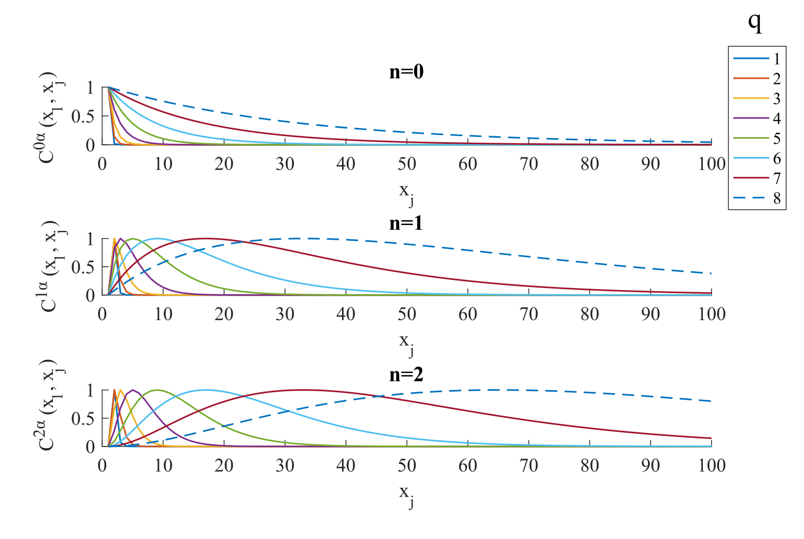
The correlation matrix V of the error term of the GLM is modelled as a linear combination of covariance components:$$$V=\sum_i\lambda_iC^i$$$. In the FAST model, a dictionary of covariance matrices with different time constants is constructed (Fig.1). These matrices are the first three terms of the Taylor expansion of exponential covariance matrices. A dictionary of length 3*p is composed of Toeplitz matrices $$$C^{n\alpha}$$$ as follows: $$C_{ij}^{n\alpha}=\begin{cases}1 & if\space j=i\space and \space n=0\\|j-i|^n e^{-\alpha|j-i|} & otherwise\end{cases} ,\space \space n\in[0,2] \space\space with \space\space \alpha=\frac{4}{2^q}$$

The ability of this model to pre-whiten data was tested on task-based fMRI data from 10 participants varying the multiband factor (1,2,4 and 8) such that TR ranged from 0.35-2.8s⁵. A factorial block design with visual stimuli of scenes and objects was used (details in ⁵). Time-series were analysed in MNI space. Motion regressors, based on the realignment, and physiological regressors, constructed from heartbeat and respiration recordings, were included in the design matrix⁶.

Given accurate estimation of the covariance matrix:

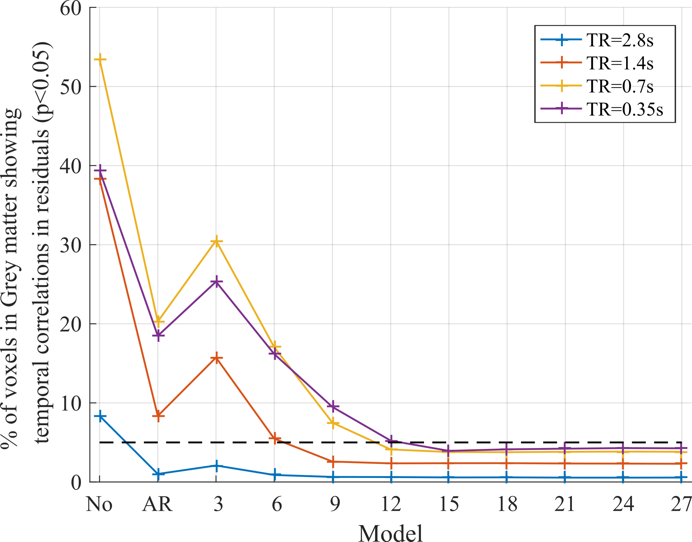
1) The residuals of the modelled time-series after pre-whitening is uncorrelated. This was tested by applying a Ljung-Box-Q test⁷ to the residuals of the first 100 time points (for consistency across TR) of each series. The dictionary of covariance components in the FAST model has size 3*p. Several GLMs were tested by varying p from 1-9. Models using the conventional AR(1)+white noise, and assuming independent samples were also tested.

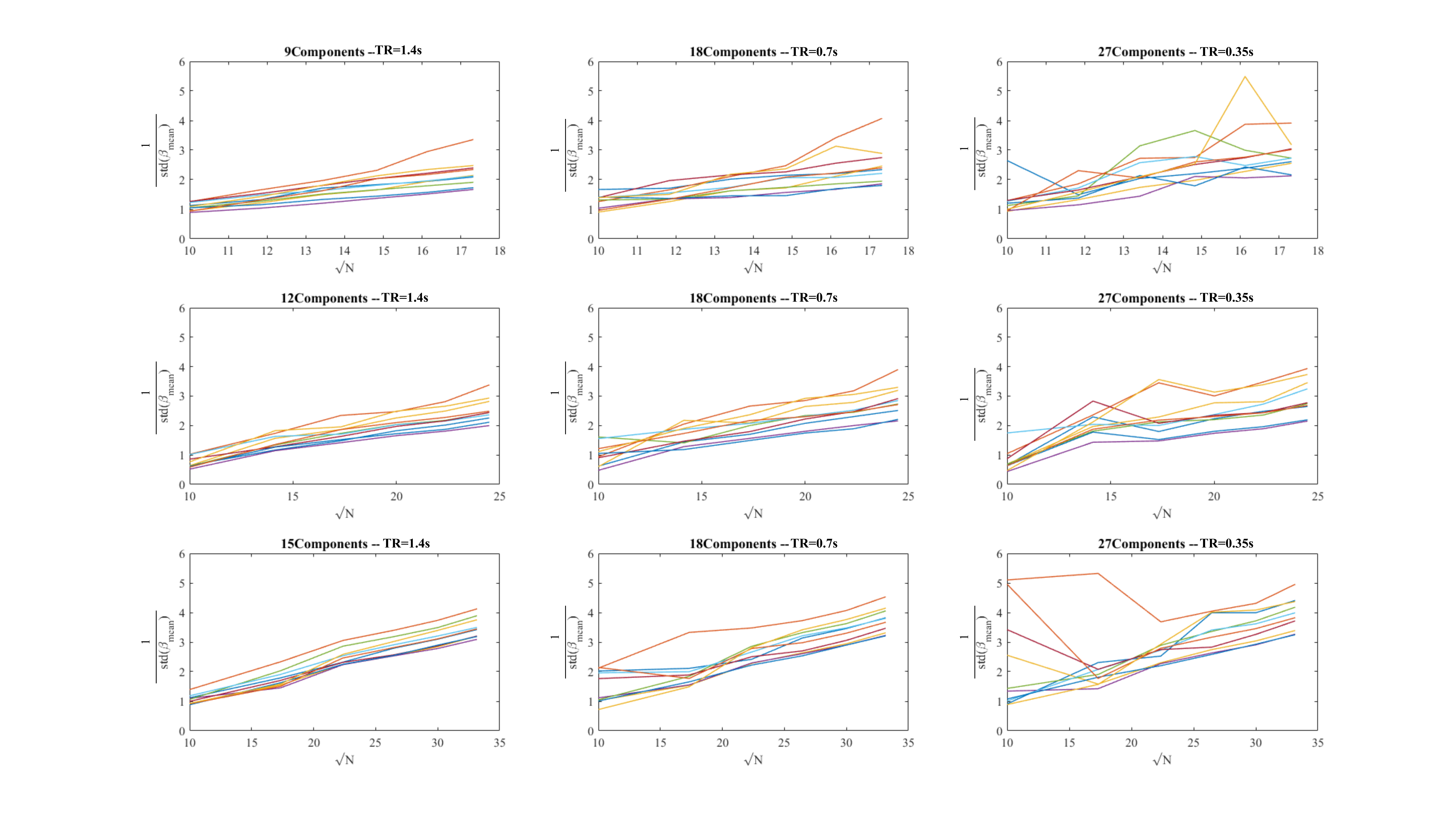
2) The standard error will depend linearly on the square root of the number of samples. This was analysed by truncating the original time-series (with TR≤1.4s to have sufficient data points).

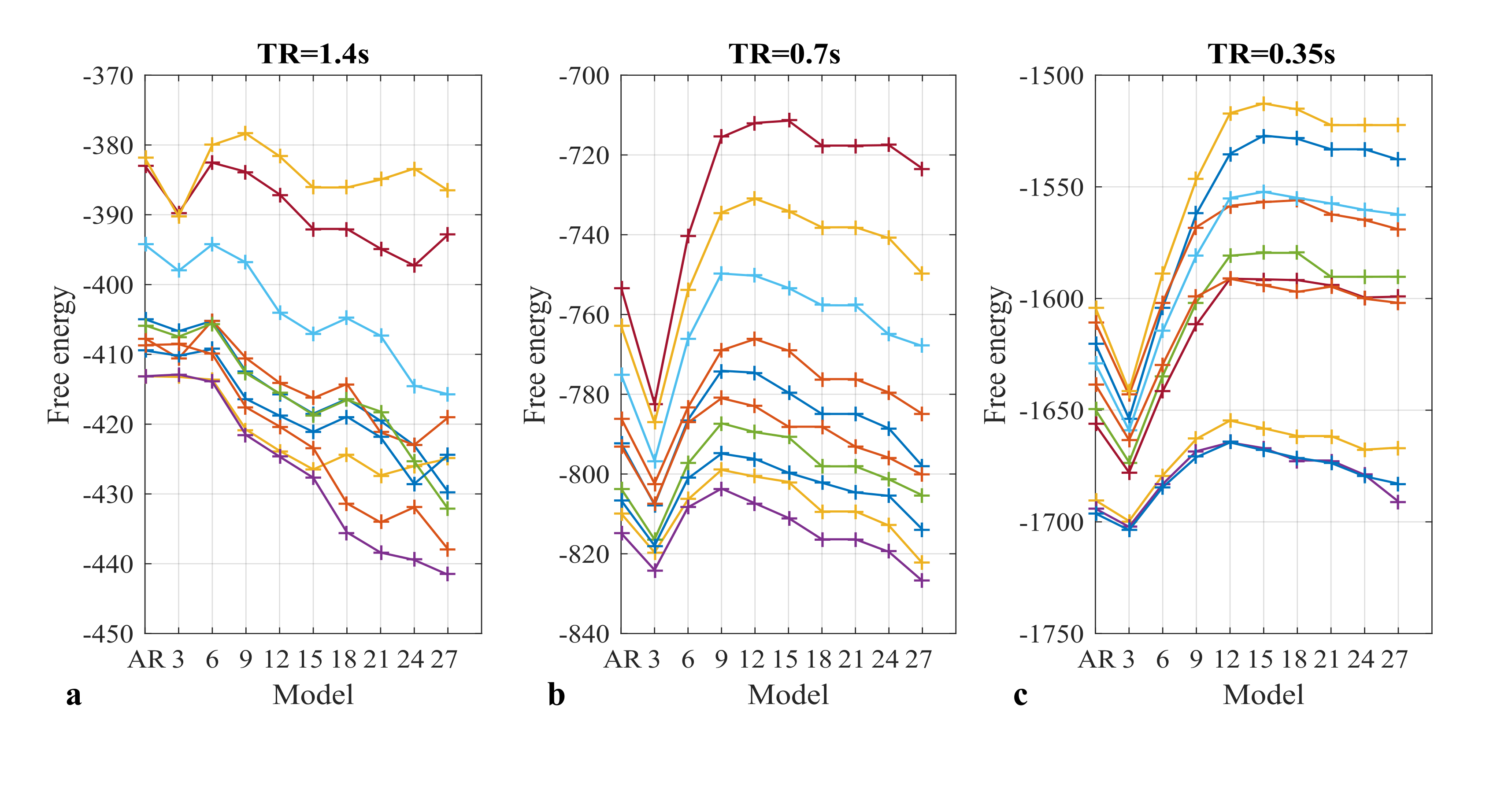
3) For a given p, ReML maximises free energy, an approximation of model evidence, accounting for both accuracy and complexity⁸, to return the optimal hyper-parameters. Therefore, maximum free energy was compared across models (for TR≤1.4s).

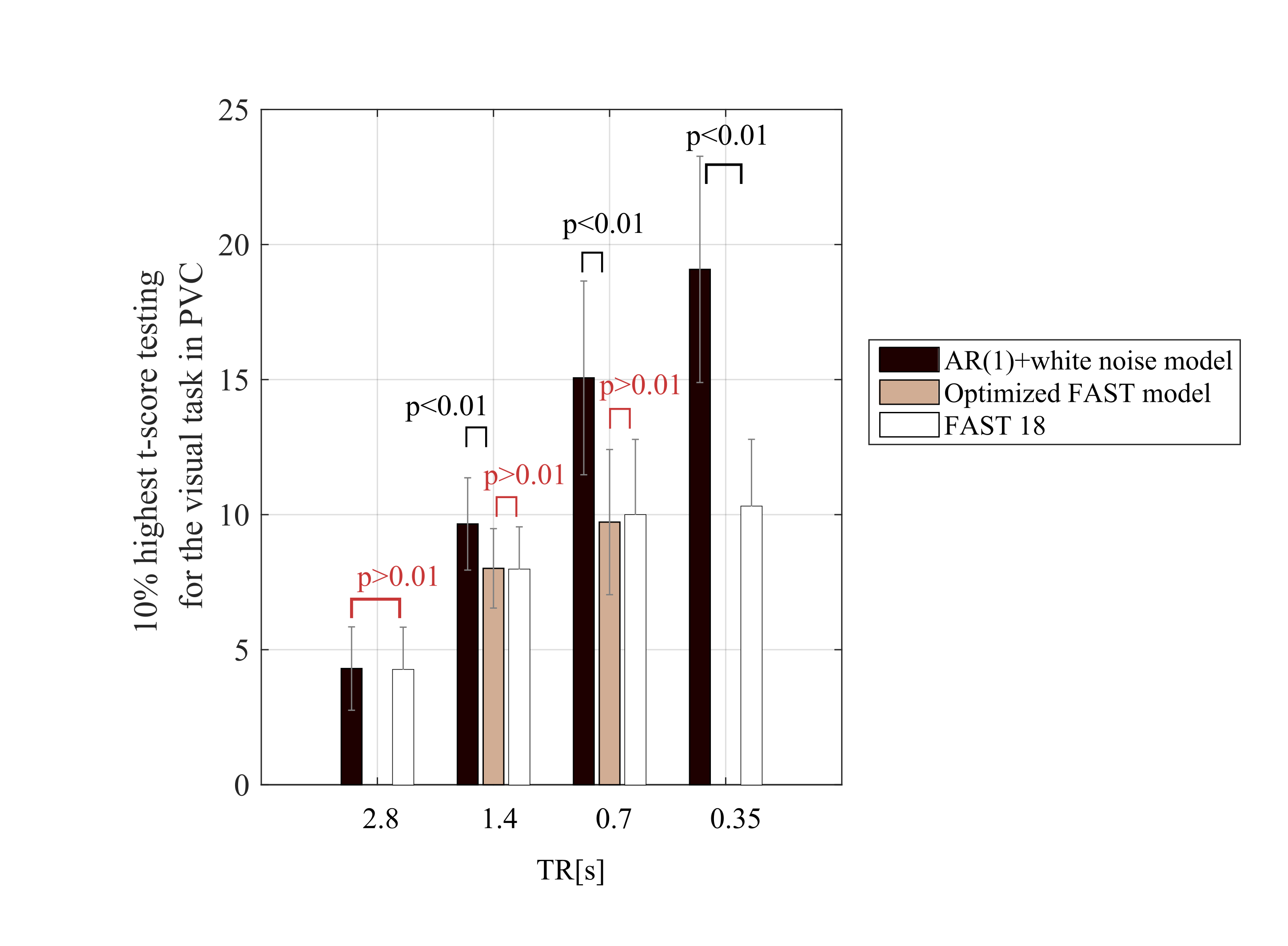
Finally, within primary visual cortex⁵, the average of the 10% highest t-scores testing for scenes versus objects was calculated with different models: AR(1)+white noise, the optimal FAST model (as per free energy analyses) and FAST with 18 components.

Results

1) While the proportion of voxels with residual correlations was dramatically decreased by the AR(1)+white noise model (Fig.2), it was insufficient for data acquired with TR≤1.4s. The minimum dictionary size required to achieve minimal temporal correlations increased with decreasing TR: 9 for TR=1.4s, 12 for TR=0.7s and 15 for TR=0.35s. Residual temporal correlations were higher for shorter TRs. However, with a dictionary size of 15 it was <5% of voxels for all TRs.

2) Using the minimum dictionary length, which achieved low-level residual correlations via Ljung-box-Q test in 1, (9 for TR=1.4s, 12 for TR=0.7s and 15 for TR=0.35s), the standard error decreased linearly with the square root of the number of samples (Fig.3). A dictionary length of 18 also ensured a linear relationship for every TR. However, when using an over-parameterised covariance model, with a dictionary size of 27, this linear behaviour was lost.

3) The dictionary length with maximum free energy was participant-specific (Fig.4). The optimal number of components increased with decreasing TR.

Finally, the t-score testing for the task was highly dependent on the model used to remove temporal correlations (Fig.5). For TR≤1.4s, the t-scores were significantly higher when calculated with an AR(1)+white noise model compared to FAST with 18 components (p<0.01). The difference between the optimal FAST model and FAST with 18 components was not significant for any TR (p>0.01).

Discussion

The FAST model is an effective means of pre-whitening rapidly sampled data. Converging results from the Ljung-Box Q test and free energy (Bayesian model comparison) analysis demonstrate that the optimal dictionary size increases with decreasing TR. Overly parameterised models (i.e., excessive dictionary sizes) should be avoided, but a reasonable dictionary size of 18 appears to be appropriate for data with TR ranging from 0.35-1.4s.

Acknowledgements

The authors would like to thank Guillaume Flandin for his valuable input regarding the interpretation of the data.

MFC is supported by the MRC and Spinal Research Charity through the ERA-NET Neuron joint call (MR/R000050/1).

The Wellcome Centre for Human Neuroimaging is supported by core funding from the Wellcome [203147/Z/16/Z].

References

[1] Friston, K. J. et al. Classical and Bayesian inference in neuroimaging: applications. NeuroImage 16, 484–512 (2002).

[2] Sahib, A. K. et al. Effect of temporal resolution and serial autocorrelations in event-related functional MRI. Magn. Reson. Med. 76, 1805–1813 (2016).

[3] Bollmann, S., Puckett, A., Cunnington, R. & Barth, M. Impact of Physiological Noise on Serial Correlations in Fast Simultaneous Multislice (SMS) EPI at 7T. in 26, 5308 (2017).

[4] Eklund, A., Andersson, M., Josephson, C., Johannesson, M. & Knutsson, H. Does parametric fMRI analysis with SPM yield valid results?—An empirical study of 1484 rest datasets. NeuroImage 61, 565–578 (2012).

[5] Todd, N. et al. Functional sensitivity of 2D simultaneous multi-slice echo-planar imaging: effects of acceleration on g-factor and physiological noise. Front. Neurosci. 11, (2017).

[6] Hutton, C. et al. The impact of physiological noise correction on fMRI at 7 T. Neuroimage 57, 101–112 (2011).

[7] Box, G. E. P. & Pierce, D. A. Distribution of Residual Autocorrelations in Autoregressive-Integrated Moving Average Time Series Models. J. Am. Stat. Assoc. 65, 1509–1526 (1970).

[8] Friston, K., Mattout, J., Trujillo-Barreto, N., Ashburner, J. & Penny, W. Variational free energy and the Laplace approximation. NeuroImage 34, 220–234 (2007).

Figures

Figure 1: Covariance components of the FAST model with p = 8

Figure 2: Proportion of voxels in which temporal correlations remained in the residuals of the GLM, with significance defined as p<0.05 with Bonferroni correction. Each data point is the average across all participants. The Ljung-Box Q test is performed with 11 different models for temporal correlations including the conventional AR(1)+white noise model (AR), No temporal correlations (No) and the FAST model with p varying from 1 to 9. The dashed line shows the threshold of 5%.

Figure 3: Relationship between the standard precision (inverse standard error) of the mean parameter testing for the constant signal and the number of samples. Temporal correlations are modelled with the 9, 18 and 27 components for TR=1.4s; 12, 18 and 27 for TR=0.7s; and 15, 18, 27 for TR=0.35s. 9, 12 and 15 are the optimal size (minimum residual temporal correlation and number of components) selected by the Ljung-Box Q test for TR=1.4, 0.7 and 0.35s respectively. Each colour represents one subject.

Figure 4: Resulting Bayesian comparison for each model (abscisses), each subject (colors) and each TR (1.4s (a), 0.7s (b), 0.35s (c)). The dictionary length with maximum free energy was participant-specific. The optimal number of components increased with decreasing TR: up to 9 components for TR=1.4s, 15 for TR=0.7s and 18 for the shortest TR (0.35s).

Figure 5: Variation of the 10% highest t-score testing for the task in the primary visual cortex with respect to TR and the model used for accounting for temporal correlation. The bar represents the mean across participants and the black line represents the standard deviation across participants. The optimized FAST model is 9 for TR=1.4s, 15 for TR=0.7s and 18 for 0.35s, according to the Bayesian comparison analysis.

Proc. Intl. Soc. Mag. Reson. Med. 26 (2018)

5473