5462
Mouse auditory pathway mapping using BOLD fMRI coherence analysis1Champalimaud Neuroscience Programme, Lisbon, Portugal
Synopsis
The feasibility and potential of mapping the mouse auditory system through functional magnetic resonance imaging (fMRI) in mice was recently demonstrated. The goal of this work was to compare the conventional GLM analysis, which relies on the variability across regions of the haemodynamic response, with a coherence analysis, which is data-driven and provides rich temporal information. Coherence amplitudes closely follow the pattern of the GLM maps, whereas the delay maps obtained from the coherence phase show different latencies even inside each ROI. This suggests the utility of coherence analysis for mapping the auditory pathway in-vivo.
Introduction
Blood Oxygenation Level Dependent (BOLD) fMRI allows the study of widespread circuits in the brain1,2. The auditory system is highly important in the context of neuroplasticity3–6 and has been studied in the rat extensively using BOLD fMRI 5–10. However, in the mouse, auditory pathway mapping via BOLD fMRI is in its infancy11. Coherence analysis12,13 provides an excellent framework to explore fMRI data from a data-driven perspective, which benefits from independence on (1) the specific BOLD response shape and (2) its variability across regions. The objective of this work was to apply coherence analysis12,13 to task-induced BOLD auditory datasets.Methods
The setup used here was described in Ref 11. fMRI runs (12 animals, 44 runs) were performed in a blocked design fashion (15s ON-45s OFF) where stimulation consisted of pure tones presented to the animal pinna inside a 9.4T Bruker Biospec scanner equipped with a cryocoil receiver. Functional imaging was achieved through a true FISP sequence with TR/TE = 2.8/1.4 ms, slice thickness = 650 μm, in-plane resolution of 150x150 (μm)2, and a 1.307 seconds scan time per volume. All animal experiments were preapproved by the local ethics committee operating under local and EU law.
Images were preprocessed with SPM12. Different GLMs were fitted, targeting (1) a per-subject analysis and (2) a group-level analysis. A single gamma function peaking at 2.5 s was used as the haemodynamic response.
Coherence analysis was computed in an ROI basis, each ROI to all the rest, and also voxelwise. For the latter each voxel’s coherence was computed against the timecourse of a seed ROI, the cochlear nucleus (CN1, see Figure 2C), the first synaptic relay. In all cases the lowest frequencies of the unwrapped coherence phase were fitted to a regression model whose slope provided the delay in seconds to the considered reference. Only those voxels with a coherence amplitude over 0.4 were considered. Coherence amplitude and delay estimation were computed both for the averaged dataset and for each individual subject.
Results and Discussion
GLM analysis yielded highly significant BOLD responses (uncorrected p<0.001, t>4.40) in the vast majority of the auditory pathway’s crucial junctions (Figure 1), and the coherence amplitude maps show a strong coherence amplitude to CN1 in the same regions: CN, SOC (bilaterally), ML, LL, IC, and MGB, with the most significant activation detected in CN and in IC. The highest BOLD signal depicted by the GLM analysis is located in the inferior colliculus, whereas the highest coherence to CN1 is located in the cochlear nucleus, as expected.
Figure 2 shows coherence phase between the CN1 ROI and each other ROI. The unwrapped coherence phase (symbols), as well as the linear fits from which the delays are extracted (solid lines), are shown in Figure 2A. With the exception of AC5, all signals have negative slopes, which suggest CN activation preceded the activation in the other areas of interest. Figure 2B presents a connectivity matrix with each ROI as seed against all other ROIs, which reveals mostly positive delays (red). Except for a few exceptions which exhibited very poor BOLD contrast, the general trend observed in the ROI-based coherence analysis is an increasing delay with respect to CN1 as the pathway is traversed in the order CN-SOC-LL-IC.
Regarding the delay maps obtained from the voxelwise analysis, most of the pathway yielded positive delays with respect to CN1 (Figure 3), confirming that BOLD responses are elicited earlier in CN1. However, different latencies were observed for different regions, even within the CN1 region.
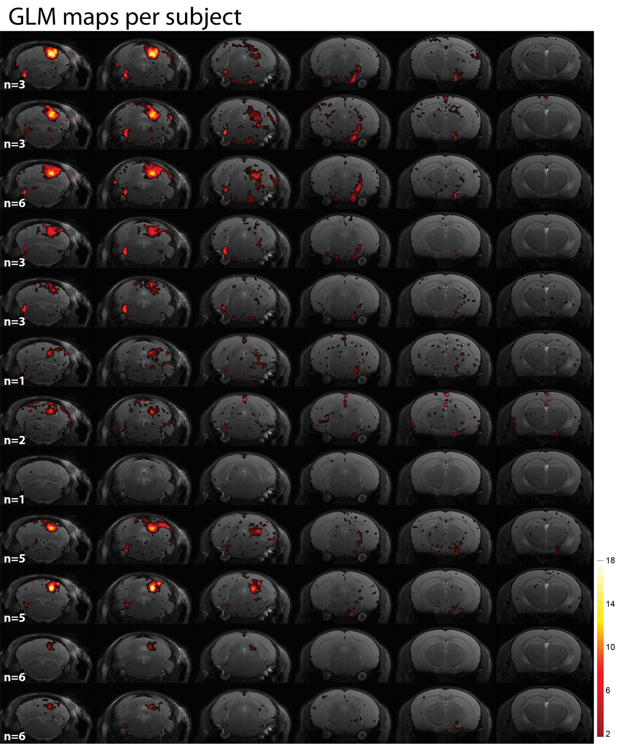
Unfortunately, Figures 4 and 5 manifest that subject-by-subject maps do not represent the whole auditory pathway, since many regions are masked out by the coherence amplitude threshold of 0.4. This is even more obvious for those subjects that underwent fewer fMRI runs, but in general the SOC (both ipsilateral and bilateral), ML and LL are not clearly represented anymore.
Conclusions
The coherence analysis proved to be a valuable alternative tool to examine BOLD data, since its amplitude closely follows that of a conventional GLM analysis, while its phase provided rich delay information even at the subregion level. The auditory pathway was delineated almost entirely except for the cortex with both analyses.
The subject-by-subject analysis evidenced the dependence of the analysis on the statistical power, since the most consistent maps correspond to those with more number of fMRI runs acquired. Thus, a study of the intersubject variability would require more extensive and balanced scanning per animal.
Acknowledgements
The authors acknowledge funding from the European Research Council (ERC) under the European Union’s Horizon 2020 research and innovation programme (Starting Grant, agreement No. 679058 and MSCA, agreement No. 753100).References
1. Logothetis NK. What we can do and what we cannot do with fMRI. Nature. 2008;453(7197):869-878. http://dx.doi.org/10.1038/nature06976.
2. Heeger DJ, Ress D. What does fMRI tell us about neuronal activity? Nat Rev Neurosci. 2002;3(2):142-151. http://dx.doi.org/10.1038/nrn730.
3. Polley DB, Steinberg EE, Merzenich MM. Perceptual learning directs auditory cortical map reorganization through top-down influences. J Neurosci. 2006;26(18):4970-4982. doi:10.1523/JNEUROSCI.3771-05.2006.
4. Yu X, Sanes DH, Aristizabal O, Wadghiri YZ, Turnbull DH. Large-scale reorganization of the tonotopic map in mouse auditory midbrain revealed by MRI. Proc Natl Acad Sci U S A. 2007;104(29):12193-12198. doi:10.1073/pnas.0700960104.
5. Lau C, Pienkowski M, Zhang JW, McPherson B, Wu EX. Chronic exposure to broadband noise at moderate sound pressure levels spatially shifts tone-evoked responses in the rat auditory midbrain. Neuroimage. 2015;122:44-51. doi:http://dx.doi.org/10.1016/j.neuroimage.2015.07.065.
6. Lau C, Zhang JW, McPherson B, Pienkowski M, Wu EX. Long-term, passive exposure to non-traumatic acoustic noise induces neural adaptation in the adult rat medial geniculate body and auditory cortex. Neuroimage. 2015;107:1-9. doi:10.1016/j.neuroimage.2014.11.048.
7. Gao PP, Zhang JW, Fan S-J, Sanes DH, Wu EX. Auditory midbrain processing is differentially modulated by auditory and visual cortices: An auditory fMRI study. Neuroimage. 2015;123:22-32. doi:http://dx.doi.org/10.1016/j.neuroimage.2015.08.040.
8. Gao PP, Zhang JW, Chan RW, Leong ATL, Wu EX. BOLD fMRI study of ultrahigh frequency encoding in the inferior colliculus. Neuroimage. 2015;114:427-437. doi:http://dx.doi.org/10.1016/j.neuroimage.2015.04.007.
9. Gao PP, Zhang JW, Cheng JS, Zhou IY, Wu EX. The inferior colliculus is involved in deviant sound detection as revealed by BOLD fMRI. Neuroimage. 2014;91:220-227. doi:http://dx.doi.org/10.1016/j.neuroimage.2014.01.043.
10. Zhang JW, Lau C, Cheng JS, et al. Functional magnetic resonance imaging of sound pressure level encoding in the rat central auditory system. Neuroimage. 2013;65:119-126. doi:10.1016/j.neuroimage.2012.09.069.
11. Blazquez Freches G, Chavarrias C, Shemesh N. Tonotopic mapping in the in vivo mouse via high resolution fMRI. In: Proceedings of the 25th Annual Meeting of ISMRM. Honolulu, Hawaii, USA; 2017.
12. Ashby FG. Coherence Analysis. In: Statistical Analysis of fMRI Data. The MIT Press; 2011.
13. Sun FT, Miller LM, D’Esposito M. Measuring interregional functional connectivity using coherence and partial coherence analyses of fMRI data. Neuroimage. 2004;21(2):647-658. doi:10.1016/j.neuroimage.2003.09.056.
Figures