5460
Correcting for the influence of cerebrospinal fluid in quantification of R2’ and deoxygenated blood volume (DBV) using quantitative BOLD1Institute of Biomedical Engineering, Department of Engineering Science, University of Oxford, Oxford, United Kingdom, 2Wellcome Centre for Integrative Neuroimaging, FMRIB, Nuffield Department of Clinical Neuroscience, University of Oxford, Oxford, United Kingdom
Synopsis
Streamlined qBOLD (sqBOLD) can be used to quantify deoxygenated blood volume and the reversible relaxation rate R2’ (used to estimate oxygen extraction fraction), although it is vulnerable to systematic errors from a number of confounding factors including the presence of cerebrospinal fluid (CSF). A FLAIR inversion preparation is typically used to null the CSF signal, but this results in a reduction in SNR, and increases scan time. We present a post-processing method to account for the presence of CSF that has the potential to improve both the accuracy and efficiency of the sqBOLD technique without the need for FLAIR preparation.
Introduction
Streamlined-qBOLD (sqBOLD)[1] uses asymmetric spin echo (ASE) data to characterise oxygen extraction fraction (OEF) and deoxygenated blood volume (DBV) in the brain, while removing confounding effects during the acquisition. The reversible transverse relaxation rate (R2′), which is used to estimate OEF, is elevated in the presence of cerebral spinal fluid (CSF)[2]. The CSF signal contribution can be nulled with a FLAIR preparation[3]. However, this limits slice coverage (due to the inversion time delay), reduces SNR (as the tissue signal has not fully recovered at inversion time), and is sensitive to motion (since slice selective inversion pulses are required). These are all important factors when applying sqBOLD to ischaemic stroke assessment[4]. This study investigates post-processing techniques for CSF signal removal that retain the rapid, self-contained nature of this methodology.Theory
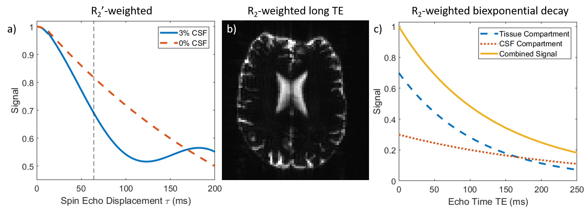
Figure 1 illustrates sources of contrast between tissue and CSF. R2'-contrast cannot be used in practice because of severe signal dropout at the large ASE offsets required to observe the CSF effect (Fig. 1a). CSF appears bright in long TE R2-weighted data, whilst tissue is dark (Fig. 1b). Finally, the large difference in R2 between CSF and tissue results in biexponential signal decay (Fig. 1c). Both R2-weighted contrast mechanisms can be used to produce maps of CSF partial volume VCSF, which can correct R2'-weighted data using Eq. 1, where \Delta\nu is the CSF off-resonance frequency shift.
$$S_{CSF}(\tau)=e^{-R_{2,CSF}TE}e^{-2\pi i\Delta\nu\tau}\tag{1}$$
Methods
Data Acquisition: Four healthy participants (mean age 28±7, 1f) were scanned using a 3T Verio system (Siemens Healthineers, Germany). For each subject, a high-resolution anatomical image was acquired, along with GESEPI-ASE scans[1] with and without FLAIR (TIFLAIR=1210ms), (FOV=240mm2, 96x96 matrix, eight 5mm (2.5mm gap) slices, TR/TE=3s/82ms, τ=-16:64ms in steps of 8ms, BW=2004Hz/px, 24s scan duration). Heavily R2-weighted data were acquired using GESEPI-ASE (TE=250ms, τ=0) for segmentation. 2D spin-echo (SE) images were acquired at 8 TEs from 66 to 248ms in steps of 26ms for biexponential fitting.
Partial Volume Estimation: R2-weighted GESEPI-ASE images were up-sampled and segmented using FAST[5]. SE data were fit for S0 and VCSF using a biexponential model, with fixed values of R2 for grey matter (12.5s-1) and CSF (4.00s-1)[6]. An R1-weighted anatomical was also segmented for comparison.
R2' and DBV Quantification: Variational Bayesian inference was performed on the ASE data using FABBER[7], with a forward model based on the three-compartment qBOLD model[8], in which the parameters S0, DBV, VCSF and R2' were inferred upon[9]. Data with FLAIR were compared with identical data acquired without FLAIR, both with and without a correction for CSF. This correction applied a high-precision prior to VCSF, with a mean based on the estimates of VCSF given by the biexponential model fit, and the R2-weighted segmentation.
Results
FLAIR SNR Cost: Without FLAIR, grey-matter SNR was 79±9; with FLAIR it was 60±5, representing approximately 25% loss of SNR.
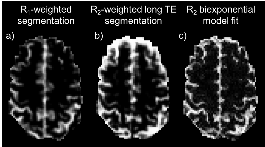
Partial Volume Estimation: Figure 2 shows example slices of the PV estimation methods: segmentation of R1-weighted MPRAGE data, segmentation of up-sampled R2-weighted SE data and a biexponential model fit of SE data. The biexponential fit appears to produce an estimate that is closer to the R1-weighted segmentation.
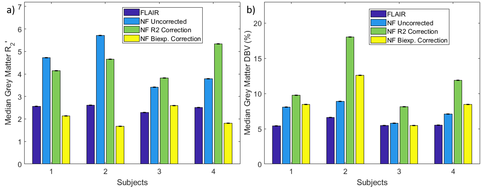
R2' and DBV Quantification: Median grey-matter R2' and DBV estimates from full model inference are shown in Figure 3. Removal of the FLAIR preparation leads to overestimation of R2', which is corrected by constraining VCSF based on partial volume estimates. Conversely, DBV is not improved by constraining VCSF in this manner. In almost all cases, the biexponential fit corrected parameter estimation more effectively than the R2-weighted segmentation.
Discussion
Segmentation of SE data, and a biexponential fit applied to SE data, produced maps of VCSF that showed considerable similarity with R1-weighted segmentation, although both tend to overestimate the amount of CSF present in voxels known to be predominantly grey matter. These methods have the advantage of having been acquired with the same distortions as the ASE data, and are already registered exactly.
Estimation of R2' is improved by constraining VCSF, with PV priors based on biexponential model fitting producing R2' estimates that were closer to the FLAIR estimates than those that used VCSF from R2-weighted segmentation. However, DBV inference is poorer when VCSF is constrained in this way, primarily because grey-matter voxels with high fractional VCSF are also inferred as having very high DBV.
Conclusion
Accounting for CSF contribution to the sqBOLD signal in post-processing, rather than by a FLAIR preparation, allows for reliable estimation of R2', and provides a potential avenue for increasing the clinical utility of the methodology. Further work is needed to ensure that DBV estimates are equally accurate after correction.Acknowledgements
This work was supported by funding from the Engineering and Physical Sciences Research Council (EPSRC) [grant number EP/K025716/1] and joint funding from the EPSRC and Medical Research Council (MRC) [grant number EP/L016052/1].References
1. Stone AJ, Blockley NP. A streamlined acquisition for mapping baseline brain oxygenation using quantitative BOLD. Neuroimage. 2017; 147:79–88.
2. Simon AB, Dubowitz DJ, Blockley NP, Buxton RB. A novel Bayesian approach to accounting for uncertainty in fMRI-derived estimates of cerebral oxygen metabolism fluctuations. Neuroimage 2016;129:198–213.
3. Hajnal JV, Bryant DJ, Kasuboski L, Pattany PM, De Coene B, Lewis PD, Pennock JM, Oatridge A, Young IR, Bydder GM. Use of fluid attenuated inversion recovery (FLAIR) pulse sequences in MRI of the brain. J Comput Assist Tomogr 1992;16:841–844.
4. Stone AJ, Harston GWJ, Carone D, Okell TW, Kennedy J, Blockley NP. Serial quantification of brain oxygenation in acute stroke using streamlined-qBOLD. bioRxiv 2017:1–31.
5. Zhang Y, Brady MJ, Smith SM. Segmentation of brain MR images through a hidden Markov random field model and the expectation-maximization algorithm. IEEE Trans. Med. Imag. 2001; 20(1):45-57.
6. Dickson JD, et al. Quantitative BOLD: the effect of diffusion. J. Magn. Reson. Imaging. 2010; 32(4):953–61.
7. Chappell MA, et al. Variational Bayesian Inference for a Nonlinear Forward Model. IEEE Trans. Signal Process. 2009; 57(1):223–36.
8. He X, Yablonskiy DA. Quantitative BOLD: Mapping of human cerebral deoxygenated blood volume and oxygen extraction fraction: Default state. Magn. Reson. Med. 2007; 57(1):115–26.
9. Cherukara MT, et al. Bayesian Inference of Brain Oxygenation and Deoxygenated Blood Volume in Acute Stroke using Streamlined Quanitative BOLD. Proc ISMRM 2017, #5269.
Figures