Synopsis

Water diffusion in tissue is non-Gaussian and the expressions used to calculate diffusion parameters are approximations which introduce systematic errors dependent on the maximum b-value employed. The purpose of this study was to characterize biases in estimates of both apparent diffusion coefficient, and kurtosis and to determine their dependence on maximum b-value. Hence, equations were derived to predict biases in measured diffusion parameters and to explain much of the discrepancy between measurements obtained with different b-values. The equations may also be used to choose appropriate maximum b-values for diffusion-weighted, tensor, and kurtosis imaging.

Introduction

The signal generated in a diffusion-weighted MRI sequence is given by [1, 2]

$$ S=S_{0}e^{a_{1}bD+a_{2}b^{2}D^{2}+a_{3}b^{3}D^{3}+...} (1)$$

where S₀ is the signal without diffusion weighting, a_i are a series of numerical coefficients, D, is the diffusion coefficient. The coefficients, a_i, depend on the probability density function describing diffusion. In bulk fluids, diffusion is Gaussian, a₁=1, and a_i>1=0

$$ S=S_{0}e^{-bD} (2)$$

For non-Gaussian diffusion, the signal is better described by [1, 2],

$$ S=S_{0}e^{-bD+\frac{Kb^{2}D^{2}}{6}+O(b^{3}D^{3})} (3)$$

Diffusion parameters are measured by acquiring images at different b-values and fitting one of these models to diffusion signal using non-linear least squares algorithms. Errors in estimates are due both to thermal noise in the signal and to biases due to failure to take the higher order terms into account. To measure kurtosis, relatively high b-values are required. As b_max increases, bias in estimates increases due to the increasing influence of higher order terms. It has been recommended that for kurtosis imaging, b_max should be less than 3/DK, the point at which signal no longer monotonically decreases. Here, an alternative maximum b-value criterion is derived.

Methods

This study was approved by the relevant institutional review board. A healthy volunteer underwent a multi b-value DWI brain scan using a 3 T Siemens Prisma scanner. Imaging parameters were: nine b-values 0-3000 smm^-2; total slices, 68; diffusion directions, 30; FOV, 256×256 mm²; voxel size: 2×2×2 mm³; TR/TE, 9000/90 ms.

Diffusion Weighted Bias

Analytical expressions were derived for the bias in estimates of D of Eq. (2) and in D and K of Eq. (3). These expressions allowed quantitative assessment of estimation biases for two b-values, b_min and b_max. The estimate of D was

$$\tilde{D}=-\frac{ln(S(b_{max})/S(b_{min}))}{b_{max}-b_{min}}\approx D-\frac{KD^{2}(b_{max}+b_{min})}{6} (4)$$

where we assumed that the higher order terms of Eq. (1) are dominated by kurtosis. Fractional errors caused by using very high maximum b-values are

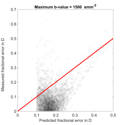
$$e_{D}=\left | {\frac{\tilde{D}-D}{D}} \right |=\frac{DK(b_{max}+b_{min})}{6} (5)$$

Diffusion Kurtosis Bias

Calculation of the bias in kurtosis measurements requires calculation of the third order term in Eq. (1), corresponding to the sixth moment of diffusion. Following the approach of Jensen et al., the 6^th moment, L, is [5]

$$L=\frac{\langle\bf ( {n.s})^{\tt {6}} \rangle}{\langle \bf ( n.s)^{\tt 2} \rangle^{\tt 3}}-15\frac{\langle \bf (n.s)^{\tt 4} \rangle}{\langle \bf (n.s)^{\tt 2} \rangle^{\tt 2}}+30 (6)$$

where s is net displacement vector, and n is the unit vector in the direction of interest. Including L in the Taylor expansion of the diffusion signal gives

$$ ln(S(b)/S_{0})=-bD+\frac{Kb^{2}D^{2}}{15}+\frac{Lb^{3}D^{3}}{90}+O(b^{4}) (7)$$

where the additional term has been derived by a simple extension of the method given in [1].

For free (Gaussian) diffusion, L, like K, is zero. For a box-car distribution corresponding to diffusion in an impermeable cavity of radius small compared with the diffusion distance, L is 48/7. By comparison, D=r²/6T_TD, where r is the radius of the cavity, T_TD is the total diffusion time, and K = -1.2 [6]. If three b-values (0, bmax/2 and bmax ) are used, it could be shown that D and K are estimated by [2]

$$ \tilde{D}=2Q_{1}-Q_{2}, \tilde{K}=12\frac{Q_{1}-Q_{2}}{b_{max}\tilde{D}^{2}} (8)$$

where

$$Q_{1}=\frac{2ln(S_{0}/S_{1})}{b_{max}}, Q_{2}=\frac{ln(S_{0}/S_{2})}{b_{max}} (9)$$

and S₁ and S₂ are the signals acquired with b = b_max/2 and b = b_max, respectively. The biases are:

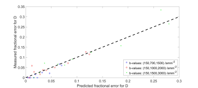
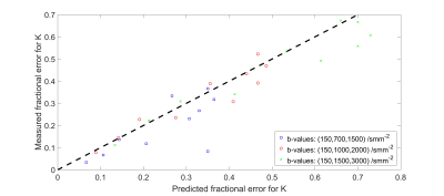
$$e_{D}=\left | {\frac{\tilde{D}-D}{D}} \right |=\frac{D^{2}Lb_{max}^{2}}{180}, e_{K}=\left | {\frac{\tilde{K}-K}{K}} \right |=\frac{DLb_{max}}{10K}, (10)$$

where we have assumed negligble errors for D to calculate e_K.

These expressions allow estimating the maximum b-value to avoid the bias of greater than a specified fraction. For organs with high diffusion anisotropy such as white matter, maximum b-value should be chosen on the basis of the highest directional DK (for Gaussian), or DL or D²L (for non-Gaussian). Since axonal direction is not known a priori, it is necessary to apply this value in all gradient directions. This may be of particular importance in estimates rooted in diffusion models.

Results

DWI

Figure 1 gives plots of measured fractional error in D vs. fractional error of Eq. (5).

DKI

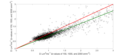
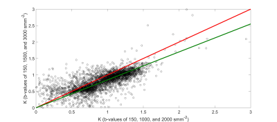
Figures 2, and 3 give plots of measured fractional errors vs. fractional errors of Eq. (10) for D, and K, respectively. Figures 4, and 5 gives plots of D, and K derived using different maximum b-values, respectively.

Discussion

Conclusion

Acknowledgements

References

1. Jensen, J.H., et al., Diffusional kurtosis imaging: the quantification of non-gaussian water diffusion by means of magnetic resonance imaging. Magn Reson Med, 2005. 53(6): p. 1432-40.

2. Jensen, J.H. and J.A. Helpern, MRI Quantification of Non-Gaussian Water Diffusion by Kurtosis Analysis. NMR in biomedicine, 2010. 23(7): p. 698-710.

3. Gilani, N., P.N. Malcolm, and G. Johnson, Parameter Estimation Error Dependency on the Acquisition Protocol in Diffusion Kurtosis Imaging. Appl Magn Reson, 2016. 47(11): p. 1229-1238.

4. Gilani, N., et al., Minimization of errors in biexponential T2 measurements of the prostate. J Magn Reson Imaging, 2015. 42(4): p. 1072-7.

5. Grinstead, C. and J. Snell, Introduction to probability. 2012: American Mathematical Society.

6. Gilani, N., P. Malcolm, and G. Johnson, A monte carlo study of restricted diffusion: Implications for diffusion MRI of prostate cancer. Magn Reson Med, 2017. 77(4): p. 1671-1677.

7. Lanzafame, S., et al., Differences in Gaussian diffusion tensor imaging and non‐Gaussian diffusion kurtosis imaging model‐based estimates of diffusion tensor invariants in the human brain. Medical physics, 2016. 43(5): p. 2464-2475.