Synopsis

Diffusion-weighted imaging with high b-value can potentially capture the restricted diffusion in tissues. With high-b-value diffusion weighting, the signal in tissue decays non-exponentially, thus the expansion of DWI signal usually be interpreted at second order or higher. However, in the ultra-high b-value (b>4k s/mm²), the cumulant expansion of higher order would fail to fit the signal. In this study, DTI, DKI, biexponential and Kärger models were used for approximating DWI signals with ultra-high b-values.

Introduction

In the diffusion-weighted imaging (DWI), changes of diffusion signal reflect histological properties of the cells, and use of a higher b-value can potentially capture more restricted diffusivity tissues, such as the heterogeneous cellula in glioma¹. Development of modern gradient systems enables producing large diffusion gradients with less eddy current, to achieve a b-value up to 10k s/mm² with an acceptable TE and SNR for a clinical exam. With high diffusion weighting, the signal in tissue decays non-exponentially, thus the expansion of DWI signal is interpreted with a biexponential model or at second order or higher. However, in the ultra-high b-value (b>4k s/mm²), the cumulant expansion of higher order would fail to fit the signal².

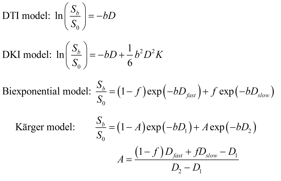
In this study, to fit the curve of DWI signal with b-values from conventional (b=1k s/mm²), up to ultra-high value (b>4k s/mm²), a linear model as for DTI, a second-order model as for DKI³, and biexponential models^4–6 without and with exchange between the intracellular and extracellular water were used and compared.

Methods

Data acquisition was performed on a MAGNETOM Prisma 3T scanner using a 64-channel head-neck coil (Siemens Healthcare, Erlangen, Germany). A healthy volunteer (27 years old) was scanned. The DWI images were obtained using a prototype simultaneous-multi-slice diffusion EPI sequence⁷ (TR/TE=3000/104 ms, voxel size=2x2x5mm³, slice number=27, bandwidth=2272 Hz/Px, partial Fourier=6/8, iPAT factor=2, SMS factor=3, TA=6min17sec). The diffusion scheme contained 20 directions for each b-value (1k, 2k, 4k, 6k, 8k and 10k s/mm²) with one non-diffusion image.

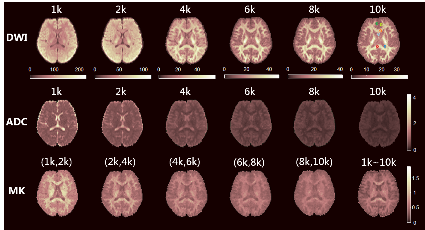
ADCs were calculated from each single b-value data. Mean kurtoses (MK) in DKI model were calculated using the DKE software⁸ from six DWI datasets, which were selected from the data with different b-value groups, noted as (1k,2k), (2k,4k), (4k,6k), (6k,8k), (8k,10k), and the full DWI data from the six datasets. The biexponential model was based on the two-component assumption with fast and slow diffusivities. For the relatively long diffusion time of 51 ms in the sequence, the exchange of water between the two components was considered in the Kärger model, but the T2 effect was not included in this study. The parameters of these two models were estimated using a nonlinear fitting. The signal attenuation of the four models are shown in Figure 1. Then the signal approximation of each model was performed from the datasets of (1k,2k), (8k,10k) and full DWI, with the b-values from 0 up to 10k s/mm². Six representative voxels were chosen from white matter, gray matter and CSF for the comparison.

Results and Discussion

As shown in Figure 2, with an increase of b-value, the signal of gray matter reduces more rapidly than that of white matter in the DWI images. The ultra-high DWI can thus potentially highlight anisotropic tissues like white matter. The ADC in the DTI model also changes a lot as the compartment of fast diffusivity is vanishing with ultra-high diffusion weighting. The MK generated from each DWI group changed relatively more mildly with b-values, but still shows a difference in the full DWI group, where the boundaries of white matter and gray matter are better recognized.

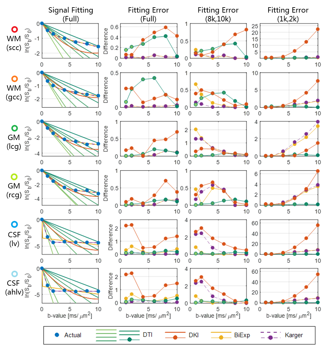
The fitting curve and errors of four models with actual DWI signal are plotted in Figure 3. The ADCs in the linear DTI model only fit well under the identical b-value due to its linear assumption, thus the related fitting errors at each b-value can be a ‘reference’ for comparison. In the (1k,2k) DWI dataset, all the models fit well when the b-value is lower than 4k s/mm², and increase substantially in the high b-value in all voxels (third column). For the DKI model, the second term is proportional to the square of the b-value, thus the fitting error increased rapidly. For the two bi-exponential models, components with fast diffusivity occupy the signal decay in the low b-values. And in the (8k,10k) DWI dataset, the fittings show reverse tendency along the b-value. Because the signal of the fast diffusion component has vanished completely therefore revealed the restricted diffusion component. Moreover, in the full DWI data, the Kärger model and biexponential model are overlapped, both of them show good fitting in white matter and gray matter. In the CSF, the Kärger model fits better than the conventional biexponential model. And the DKI model could not fit well in all the b-values.

Conclusion

Acknowledgements

References

1. Hu Y, Yan L, Sun Q, Liu Z, Wang S. Comparison between ultra-high and conventional mono b-value DWI for preoperative glioma grading. Oncotarget. 2017;8(23):37884-37895.
2. Kiselev VG. The cumulant expansion: an overarching mathematical framework for understanding diffusion NMR. Diffus MRI theory, methods, Appl. 2010;2(1):152-168.
3. Jensen JH, Helpern JA, Ramani A, Lu H, Kaczynski K. Diffusional kurtosis imaging: The quantification of non-Gaussian water diffusion by means of magnetic resonance imaging. Magn Reson Med. 2005;53(6):1432-1440.
4. Assaf Y, Cohen Y. Non-mono-exponential attenuation of water and N-acetyl aspartate signals due to diffusion in brain tissue. J Magn Reson. 1998;131(1):69-85.
5. Niendorf T, Dijkhuizen RM, Norris DG, van Lookeren Campagne M, Nicolay K. Biexponential diffusion attenuation in various states of brain tissue: implications for diffusion-weighted imaging. Magn Reson Med. 1996;36(6):847-857.
6. Kärger J, Harry P, Wilfried H. Principles and Application of Self-Diffusion Measurements by Nuclear Magnetic Resonance. Adv Magn Opt Reson. 1988;12(C):1-89.
7. Setsompop K, Gagoski BA, Polimeni JR, Witzel T, Wedeen VJ, Wald LL. Blipped-controlled aliasing in parallel imaging for simultaneous multislice echo planar imaging with reduced g-factor penalty. Magn Reson Med. 2012;67(5):1210-1224.
8. Tabesh A, Jensen JH, Ardekani BA, Helpern JA. Estimation of tensors and tensor-derived measures in diffusional kurtosis imaging. Magn Reson Med. 2011;65(3):823-836.