Synopsis

Characterizing uncertainty distributions in diffusion MRI derived metrics such as fractional anisotropy or kurtosis anisotropy requires non-parametric approaches, since the correct form of the distribution is rarely known a priori. Previously suggested wild bootstrapping methods, however, have not considered the impact of outliers in the data. In this work, we updated the existing wild bootstrap methodology to consider outliers detected by a robust model estimator, adopting a strategy similar to the rejection of the outliers prior to the model estimate. Additionally, we used simulations based on real human data to demonstrate the benefits of our pipeline for recovering uncertainty distributions.

Introduction

Metrics estimated from diffusion MRI¹ (dMRI) can characterize underlying tissue microstructure. For example, diffusion tensor imaging² (DTI) and diffusion kurtosis imaging³ (DKI) are used to obtain metrics such as fractional anisotropy (FA)⁴, kurtosis anisotropy (KA)⁵ and diffusion orientation information, which have been studied extensively in health and disease.

dMRI measurements, however, are affected by noise and various artefacts⁶ that hinder the accurate determination of derived metrics. Wild bootstrapping⁷ (WB) which considers the heteroscedasticity of dMRI data has been suggested to provide the empirical means to study such unknown distributions^8,9. In addition to heteroscedasticity, the presence of outliers can significantly bias the estimation on which bootstrapping is based if not handled appropriately. Although robust estimators in the presence of homoscedastic and heteroscedastic errors have been proposed^10,11, they have not been used in bootstrapping strategies to date.

Here, we present a wild robust bootstrap (ROBOOT) approach, in which bootstrap samples are based only on model residuals corresponding to the measurements not identified as outliers by a robust model estimator¹⁰. Differences between the ‘standard’ wild bootstrapping and ROBOOT are demonstrated with simulations, demonstrating an improved precision of the tensor first eigenvector, FA, and KA estimates when using ROBOOT.

Methods

Simulations

dMRI data from the MASSIVE database¹³ were used to estimate the DKI-model, and a ground truth (GT) dataset was created from the estimated DT and KT. The GT consisted of two 60-direction shells with b-values 1000s/mm² and 2000s/mm² along with 5 non-diffusion weighted signals.

A ‘baseline simulation’ without outliers was generated by introducing Rician noise with signal-to-noise ratio (SNR) of 32 to the GT DWIs, and used to study the variability in estimates due to noise effects. In addition, outlier simulations with interleaved artefacts (Fig 1a) were generated by randomly replacing 5% of the DWIs by artefactual volumes with 50% signal decrease before introducing Rician noise with SNR 32.

Tensor estimation

Tensor estimates, of which the components are represented in the matrix $$$\hat{\mathbf{d}}$$$, were obtained using the iteratively re-weighted linear least squares (IWLLS)^14–16 estimator for both the baseline- and outlier simulations. In addition, REKINDLE was used to obtain estimates in the outlier simulations¹⁰ to flag outliers that were input to the ROBOOT-framework.

Bootstrapping

The wild bootstrap⁷ samples $$$y_{i}^{*}$$$ (eq.1) for $$$\text{DWI}_i$$$ ($$$i=1,...,N$$$) were generated as described in⁸ with the addition of KT elements in $$$\hat{\mathbf{d}}$$$:

$$y_{i}^{*}=\left( X \hat{\mathbf{d}} \right)_{i} + a_{i} u_{i} \epsilon_{i}^{*} , \tag{1}$$

where $$$X$$$ is the design matrix, the heteroscedasticity consistent covariance matrix estimator $$$a_{i}=\sqrt{\frac{1}{1-h_{i}}}$$$ is the $$$i$$$th diagonal of $$$H= X \left( X^{T}X \right)^{-1} X^{T}$$$, $$$u_{i}$$$ is the residual of the original model estimation, and $$$\epsilon_{i}^{*}$$$ is drawn from the the auxiliary distribution^7,17 (eq.2):

$$F_{1}: \quad \epsilon_{i}^{*} = \left \{ \begin{array}{l} 1, \quad \text{with 50% probability} \\ -1, \quad \text{with 50% probability} \end{array} \right .\tag{2}$$

ROBOOT was implemented by removing the residuals, $$$u_{i}$$$ , and respective rows, $$$X_i$$$ detected as outliers with REKINDLE. This ensured that the bootstrap sample would not be affected by the erroneous measurements, thus representing the uncertainty of the robust model estimate.

Results

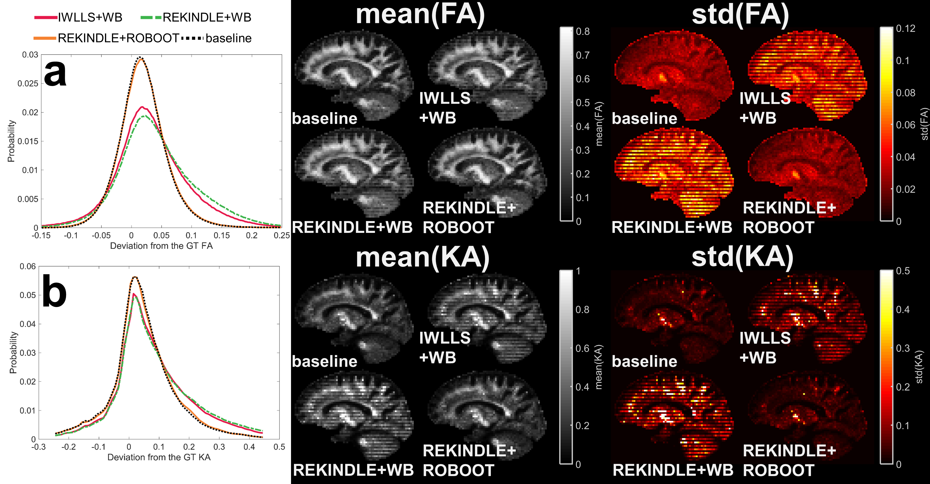
Figure 1 shows the deviations from the GT FA (a) and KA (b) for the sagittal slice simulation based on 1000 bootstrap samples. The REKINDLE-based ROBOOT produced nearly identical results compared to the baseline simulation. Slice visualizations of the mean and standard deviation FA and KA values show the standard wild bootstrap approach is affected by the interleaved artefact whereas the ROBOOT distribution features are similar to the baseline.

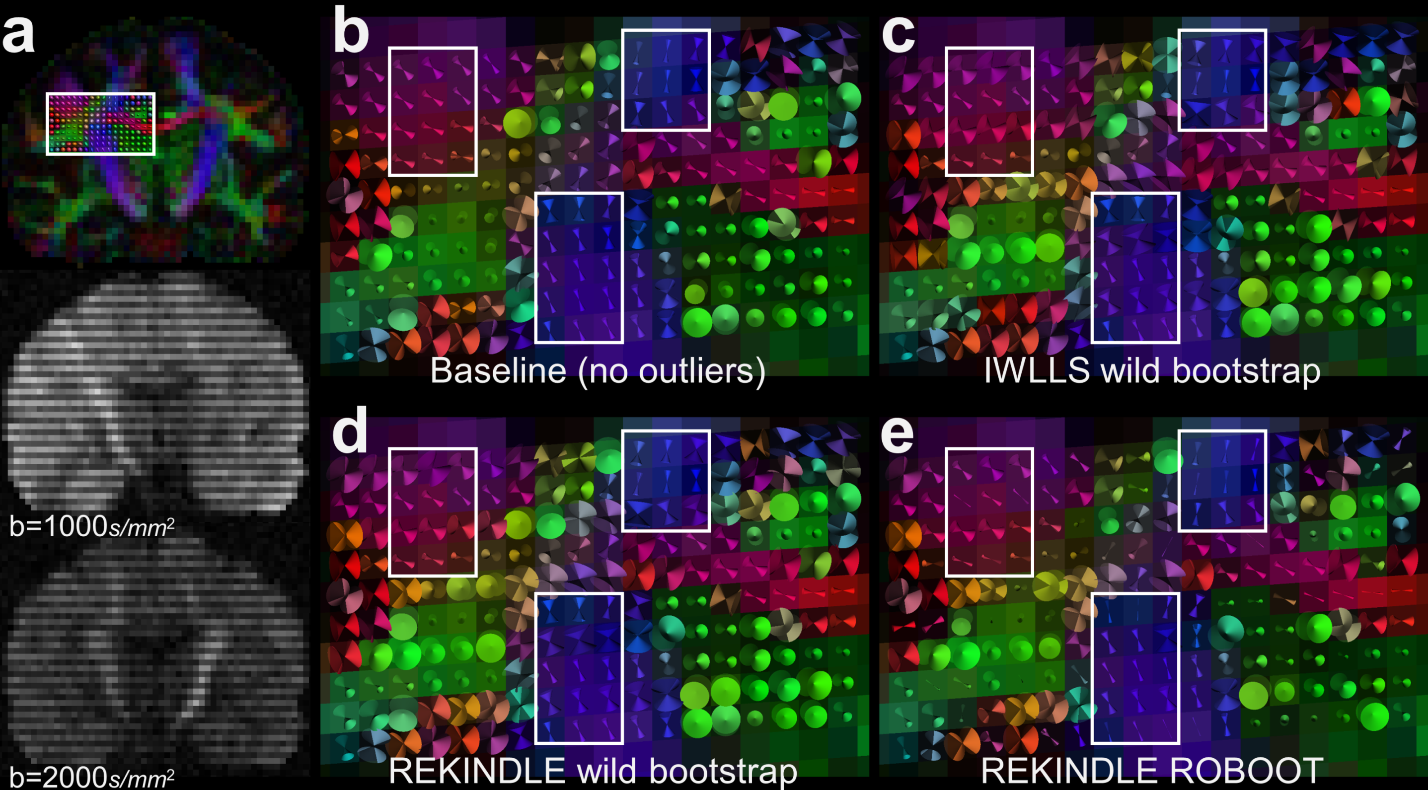
Figure 2 a shows a coronal slice from the GT color-coded FA image and the interleaved signal artefact on two DWIs. The white box in a highlights the Region-of-Interest used to visualize Cone-of-Uncertainty (CoU) values determined using 1000 bootstrap samples. b visualizes the baseline CoUs (no outliers simulated). c shows IWLLS estimation combined with the wild bootstrap, in which case both the orientation of the cone (i.e. orientation of DT estimate) and the cone’s solid angle (uncertainty) are affected. In contrast, with the REKINDLE-based wild bootstrap (d) only the uncertainty is affected. Finally, when using REKINDLE with ROBOOT, the uncertainties are decreased to a similar level as the baseline simulation. The most distinct differences are highlighted in white squares.

Conclusion

Acknowledgements

References

1. Stejskal, E. O. & Tanner, J. E. Spin Diffusion Measurements: Spin Echoes in the Presence of a Time‐Dependent Field Gradient. J. Chem. Phys. 42, 288–292 (1965).

2. Basser, P. J., Mattiello, J. & LeBihan, D. MR diffusion tensor spectroscopy and imaging. Biophys. J. 66, 259–67 (1994).

3. Jensen, J. H., Helpern, J. A., Ramani, A., Lu, H. & Kaczynski, K. Diffusional kurtosis imaging: The quantification of non-gaussian water diffusion by means of magnetic resonance imaging. Magn. Reson. Med. 53, 1432–1440 (2005).

4. Basser, P. J. & Pierpaoli, C. Microstructural and physiological features of tissues elucidated by quantitative-diffusion-tensor MRI. J. Magn. Reson. 111, 209–219 (1996).

5. Poot, D. H., den Dekker, A. J., Achten, E., Verhoye, M. & Sijbers, J. Optimal experimental design for diffusion kurtosis imaging. IEEE Trans Med Imaging 29, 819–829 (2010).

6. Jones, D. K. & Cercignani, M. Twenty-five pitfalls in the analysis of diffusion MRI data. NMR Biomed. 23, 803–820 (2010).

7. Liu, R. Y. Bootstrap Procedures under some Non-I.I.D. Models. Ann. Stat. 16, 1696–1708 (1988).

8. Whitcher, B., Tuch, D. S., Wisco, J. J., Sorensen, A. G. & Wang, L. Using the wild bootstrap to quantify uncertainty in diffusion tensor imaging. Hum. Brain Mapp. 29, 346–362 (2008).

9. Jones, D. K. Tractography gone wild: probabilistic fibre tracking using the wild bootstrap with diffusion tensor MRI. IEEE Trans Med Imaging 27, 1268–1274 (2008).

10. Tax, C. M. W., Otte, W. M., Viergever, M. A., Dijkhuizen, R. M. & Leemans, A. REKINDLE: Robust Extraction of Kurtosis INDices with Linear Estimation. Magn. Reson. Med. 73, 794–808 (2015).

11. Chang, L. C., Walker, L. & Pierpaoli, C. Informed RESTORE: A method for robust estimation of diffusion tensor from low redundancy datasets in the presence of physiological noise artifacts. Magn. Reson. Med. 68, 1654–1663 (2012).

12. Chang, L. C., Jones, D. K. & Pierpaoli, C. RESTORE: Robust estimation of tensors by outlier rejection. Magn. Reson. Med. 53, 1088–1095 (2005).

13. Froeling, M., Tax, C. M. W., Vos, S. B., Luijten, P. R. & Leemans, A. MASSIVE brain dataset: Multiple acquisitions for standardization of structural imaging validation and evaluation. Magn. Reson. Med. 77, 1797–1809 (2017).

14. Veraart, J., Sijbers, J., Sunaert, S., Leemans, A. & Jeurissen, B. Weighted linear least squares estimation of diffusion MRI parameters: Strengths, limitations, and pitfalls. Neuroimage 81, 335–346 (2013).

15. Salvador, R. et al. Formal characterization and extension of the linearized diffusion tensor model. Hum. Brain Mapp. 24, 144–155 (2005).

16. Leemans, A., Jeurissen, B., Sijbers, J. & Jones, D. ExploreDTI: a graphical toolbox for processing, analyzing, and visualizing diffusion MR data. Proc. 17th Sci. Meet. Int. Soc. Magn. Reson. Med. 17, 3537 (2009).

17. Davidson, R. & Flachaire, E. The wild bootstrap, tamed at last. J. Econom. 146, 162–169 (2008).

18. Vorburger, R. S. et al. Insight from uncertainty: bootstrap-derived diffusion metrics differentially predict memory function among older adults. Brain Struct. Funct. 221, 507–514 (2016).