Synopsis

Diffusion-weighted imaging is a valuable asset in the diagnosis of a plethora of diseases. General guidelines are available when measuring (mono-exponential) diffusion in several organs of interest, but there is less consensus on optimal acquisition parameters for more complex models (e.g., intravoxel incoherent motion, kurtosis). We provide a general, easy to implement, solution scheme (similar to the Cramér–Rao lower bound approach) that can be used to optimize the acquisition protocol with respect to the $$$b$$$-values. We present mathematical proof, and phantom as well as in-vivo measurements that corroborate the viability of our method.

Purpose

Theory

Taking the mono-exponential model as an example, we define the model, $$$S(\beta,b)=S(0)\exp(-bD)$$$ ($$$D$$$, apparent diffusion coefficient), that describes the signal intensity decay in DWI. Here, $$$\beta=\{S(0),D\}$$$ is the list of tissue-parameters of which we presume to have best estimates $$$\overline{\beta}$$$. Second, with two measurements, of which the first is at $$$b_0=0$$$, we have a list of input parameters $$$\alpha=\{b_1,\rho_1\}$$$ to optimize our cost function. Together, these yield a list of expected measurement outcomes. A small perturbation of each of these outcomes, $$$S(b_i)\rightarrow S(b_i)+\delta S(b_i)$$$, results in a change of the estimate values of $$$\overline{D}\rightarrow\overline{D}+\delta \overline{D}_i$$$ when a form of regression is performed. We can then define the cost function $$$C =\sum_{i}\delta\overline{D}_i^2\sim\text{Var}(\overline D)$$$. In accordance with analytically known results (under assumption of constant Gaussian noise)⁴, we find optimal values at $$$\{\rho_1,b_1D\}\approx\{0.782,1.278\}$$$, or $$$b_1D\approx1.109$$$ when $$$\rho_0=\rho_1=1/2$$$ are fixed, very similar to the rule-of-thumb estimation. This approach can be generalized to a weighted squared sum over the entries of $$$\beta$$$ for any model, to include multiple tissues of interest, and more.

Methods

Using a Philips Ingenia $$$3$$$T scanner, DWI's were obtained with EPI readout.

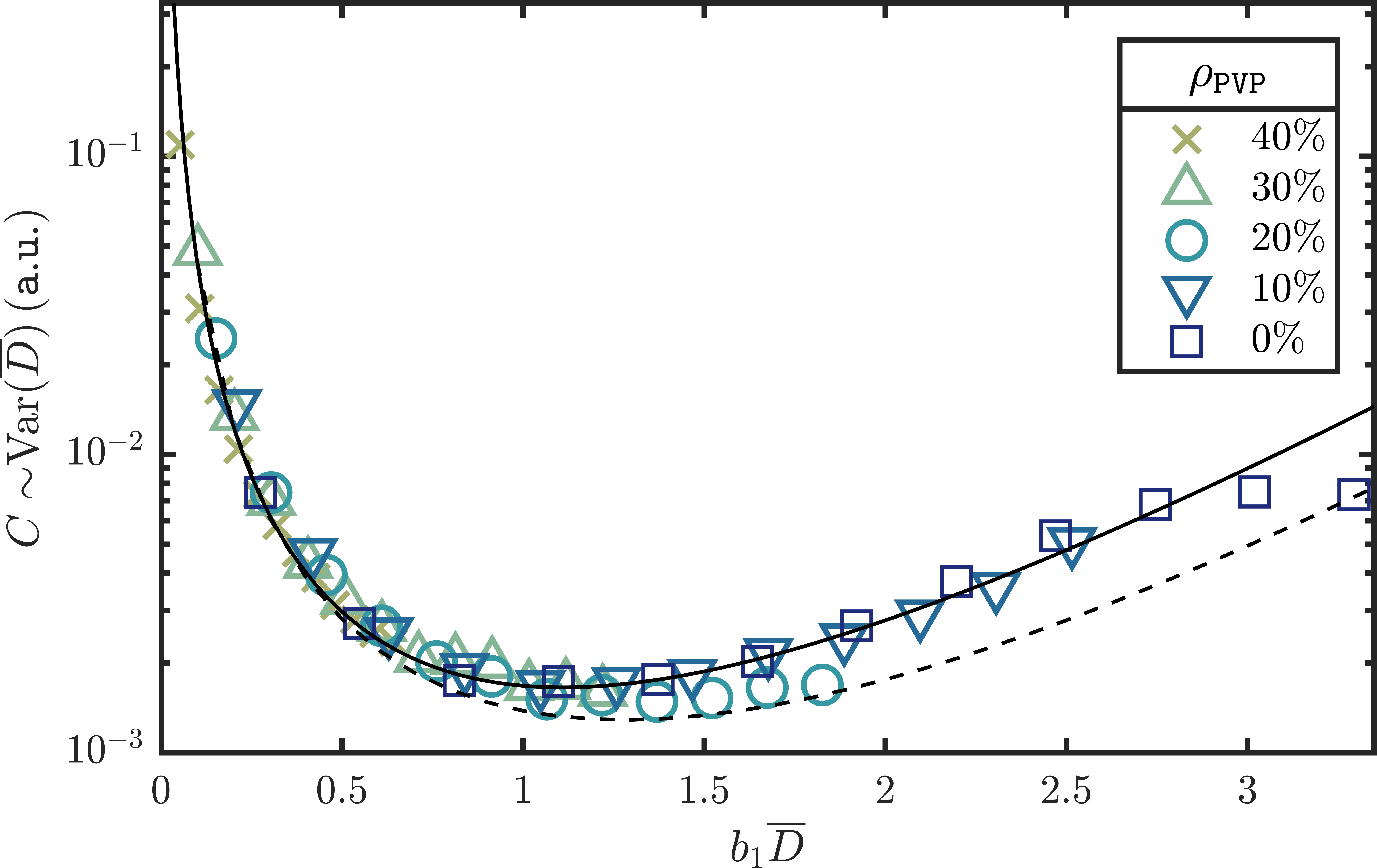
i) Using the QIBA diffusion phantom⁵ we determined $$$\overline{D}$$$, per voxel in a set of regions of interest (ROI's), by fitting an exponential through the signal at $$$b_0=0$$$ and varying $$$b_1\in\{250,500,\dots,3000\}{\tt s/mm^2}$$$. We compared $$$\text{Var}(\overline{D})$$$, as estimated from measurements, to the numerically calculated function $$$C$$$, as functions of $$$b_1$$$.

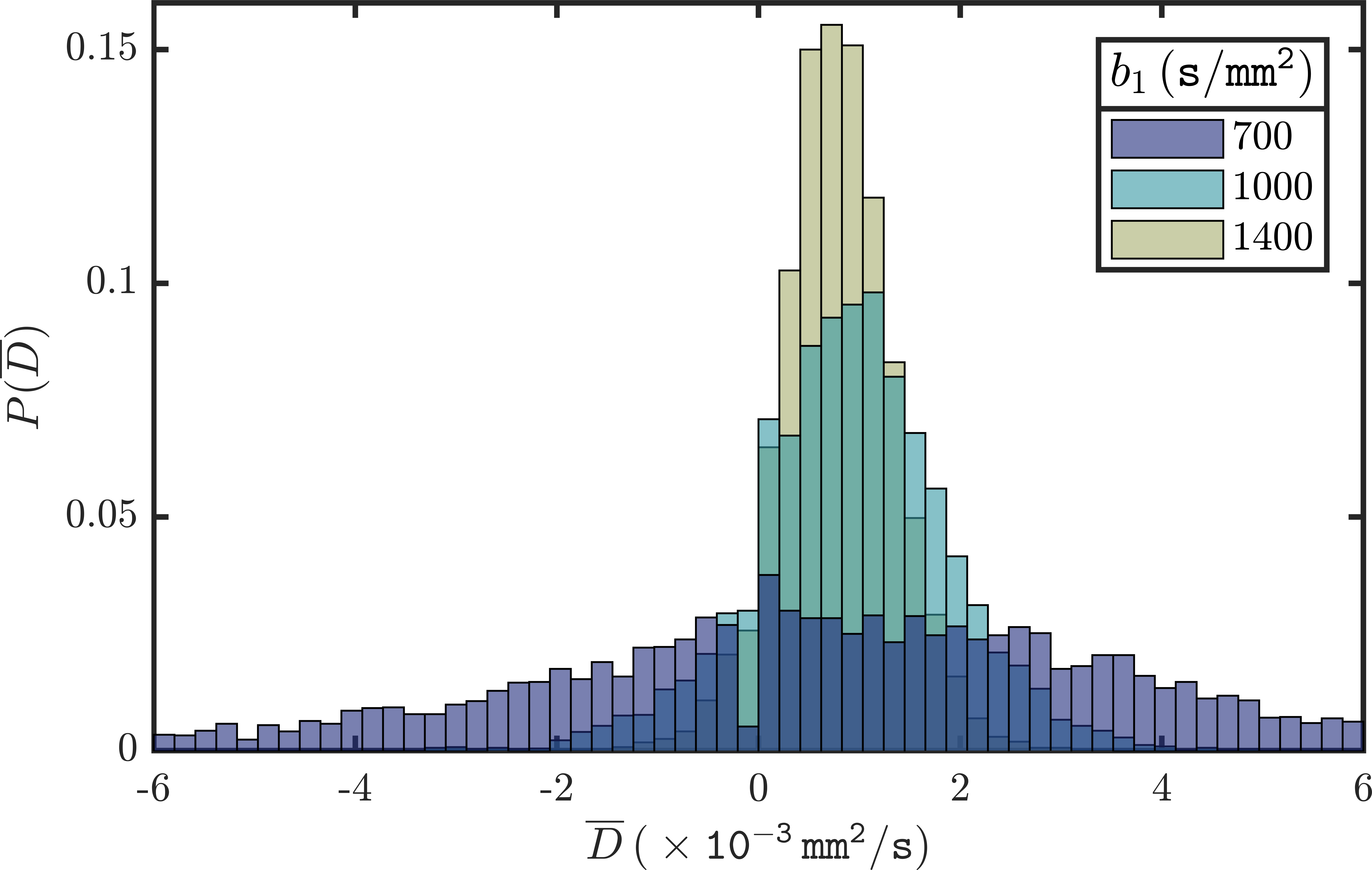
ii) In a similar fashion, we determined $$$\overline{D}$$$ in the prostate of a healthy volunteer using $$$b_0=600{\tt s/mm^2}$$$, to exclude perfusion effects, and varying $$$b_1\in\{700,1000,1400\}{\tt s/mm^2}$$$. By means of probability histograms of $$$\overline{D}$$$ the effects of $$$b_1$$$ on the width of te probability distributions, directly related to $$$\text{Var}(\overline{D})$$$, were made apparent.

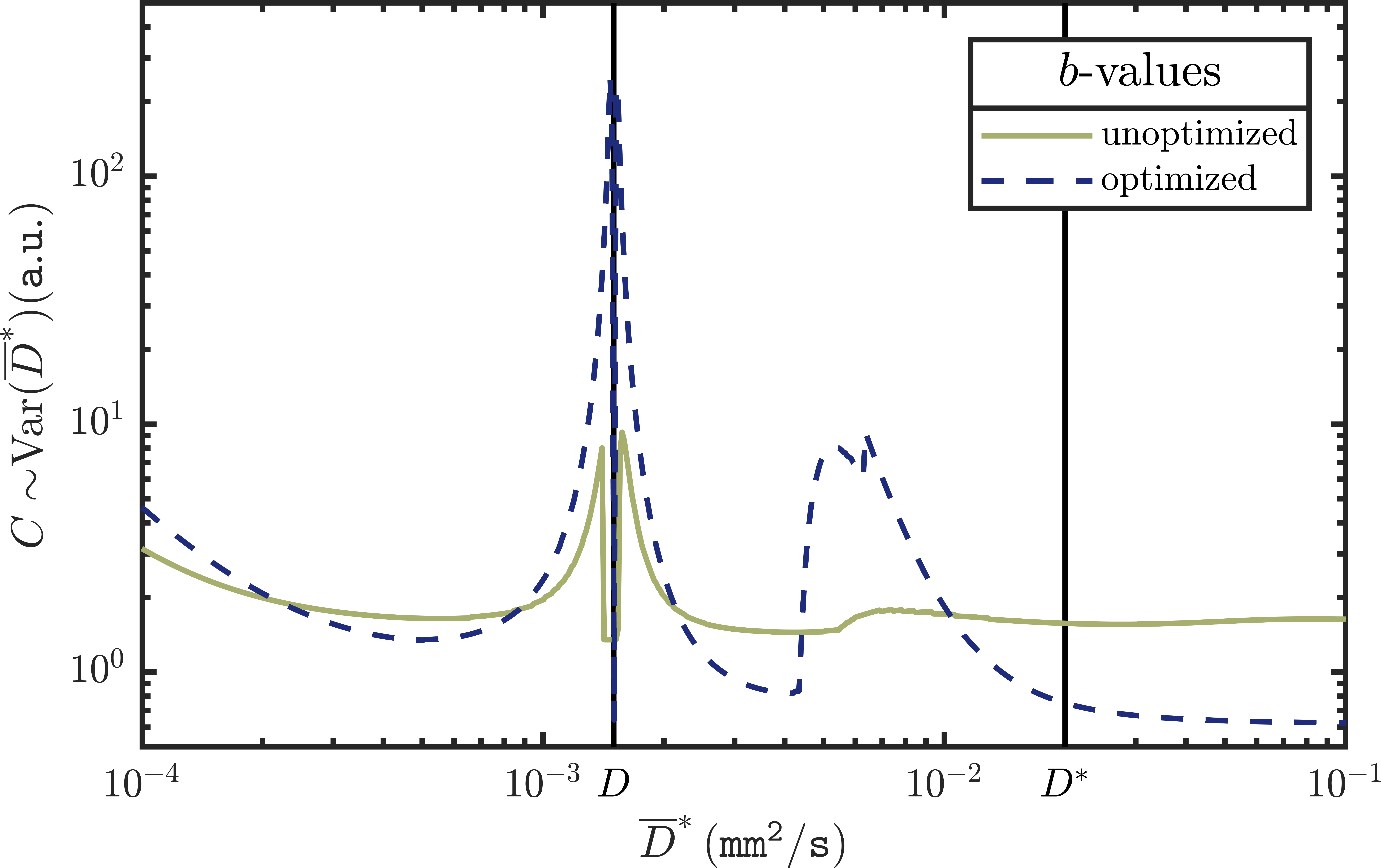
iii) By means of calculations, we numerically compared $$$C\sim\text{Var}(\overline{D}^*)$$$, for the bi-exponential model $$$S(b)/S(0)=f\exp(-bD^*)+(1-f)\exp(-bD)$$$, typically used in IVIM, with tissue parameters $$$\beta=\{S(0)=1000,f=0.1,D=0.0015{\tt mm^2/s},D^*=0.02{\tt mm^2/s}\}$$$, for an optimized and unoptimized set of $$$b$$$-values, over a range of values of $$$\overline{D}^*$$$.

Results

i) Figure 1 shows a collapse, in the high signal-to-noise (SNR, low $$$b_1\overline{D}$$$) region, of $$$C$$$ and $$$\text{Var}(\overline{D})$$$ as functions of $$$b_1\overline{D}$$$. Although $$$C$$$ is intrinsically dependent on $$$\beta=\{S(0),D\}$$$, these dependencies can be scaled out. Moreover, we apply an overall vertical rescaling per ROI, due to spatial noise variations and unknown proportionality relation $$$C\sim\text{Var}(\overline{D})$$$. This does not, however, change the minimum of $$$C$$$ with respect to $$$b$$$-values.

ii) Figure 2 shows the probability distribution of $$$\overline{D}$$$ extracted from the ROI in the prostate of a healthy volunteer. The width of the distributions are directly related to $$$\text{Var}(\overline{D})$$$ and decrease as $$$b_1$$$ approaches the optimal $$$b$$$-value.

iii) Figure 3 shows that the optimized acquisition parameters result in a lower value of $$$C$$$ at the point for which it was optimized ($$$D^*=\overline{D}^*$$$) compared to the unoptimized parameters. The drawback is that the optimized $$$C$$$ can vary (increase) more greatly away from this point.

Discussion

There are, however, also limitations to our method. At high SNR the assumption of Gaussian noise holds quite well, but at low SNR the noise is noticeably Rician in nature, and the assumption no longer holds.

Additionally, with a limited number of measurements $$$N$$$, $$$\rho_i=N_i/N$$$ can only take on a limited number of values. Although this method can be adjusted for this, it will diminish possible gains, as ideal $$$\rho$$$-values cannot be chosen, when $$$N$$$ is small (see the differences between $$$C$$$ for fixed and variable $$$\rho$$$ in Fig. 1).

Discrepancies between model and measurement can lead to significant systematic errors in the ideal acquisition parameters. Thus, care must be taken to pick a more complex model if additional effects, like slow diffusion, are to be expected. Optimization is especially important for these models (that are, generally, less robust during the fitting procedure⁶) and when acquired images are used for ADC-maps or computed DW images⁷. It is important to note that optimization schemes can also perform significantly worse if presumed tissue parameters $$$\overline{\beta}$$$ differ from the actual parameters $$$\beta$$$ (see Fig. 3).

Conclusion

Acknowledgements

References

1. A. R. Padhani et. al., Diffusion-Weighted Magnetic Resonance Imaging as a Cancer Biomarker: Consensus and Recommendations, Neoplasia 11, 102-125 (1995).

2. C. Federau, Intravoxel incoherent motion MRI as a means to measure in vivo perfusion: A review of the evidence, NMR in Biomedicine 30, e3780 (2017).

3. Y. Bito, S. Hirata, and E. Yamamoto, Optimum Gradient Factors for Apparent Diffusion Coefficient Measurements, Proc. Soc. Magn. Reson. Med. 913 (1995).

4. High Precision Devices, Inc. Quantitative (qMRI) QIBA DWI Diffusion Phantom. http://www.hpd-online.com/diffusion-phantom.php. Accessed 20-10-2017.

5. H. Merisaari et. al., Fitting methods for intravoxel incoherent motion imaging of prostate cancer on region of interest level: Repeatability and gleason score prediction, Magn. Reson. Med. 77, 1249-1264 (2017).

6. A. Ogura et. al., Optimal b Values for Generation of Computed High-b-Value DW Images, AJR 206, 713-718 (2016).