5335
The importance of constraints and spherical sampling in diffusion MRI1Department of Computer Science, University of Copenhagen, Copenhagen, Denmark
Synopsis
In this work we analyze the incidence of voxels with physically impossible model parameters, reconstructed from diffusion-weighted data that is acquired using different sampling schemes. Our results show that for cumulants up to order $$$4$$$ constrained least squares can be used to compute a reliable reconstruction of the cumulant expansion of the signal from realistic acquisitions, with spherical sampling producing fewer unsatisfied model constraints compared to space-filling sampling. Voxels where reconstruction is likely to fail are shown to be consistently localized near the white matter-gray matter interface and in deep brain structures.
Introduction
Diffusion-weighted MRI allows one to image the probability density function $$$P_\mathit{\Delta}$$$ of spin displacements (over a time $$$\mathit{\Delta}$$$) in living tissue like the human brain, providing insight into the local structure at a microscopic scale. A diffusion-weighted data set consists of a set of measurements $$$\{S_\mathit{\Delta}(\boldsymbol{q}_i)\}$$$ of the characteristic function $$$S_\mathit{\Delta}$$$ associated to $$$P_\mathit{\Delta}$$$, where $$$\boldsymbol{q} \mathrel{\mathop:}= \gamma \delta \boldsymbol{g}$$$ is the gradient wave vector defined in terms of the applied gradient vector $$$\boldsymbol{g}$$$, the pulse duration $$$\delta$$$, and the gyromagnetic ratio $$$\gamma$$$. The sampling scheme $$$\{\boldsymbol{q}_i\}$$$ is typically designed such that the data is suitable for post-acquisition processing or modeling. In this work we investigate how two commonly employed sampling strategies—space-filling sampling and spherical (shell-based) sampling—affect the degree to which necessary constraints on $$$P_\mathit{\Delta}$$$ are satisfied. We view the fraction of voxels where the constraints are satisfied as an indicator of data quality; a similar methodology has been used for example by Veraart et al.3Material and methods
The constraints we consider are derived from the convexity of the cumulant-generating function $$$\log S_\mathit{\Delta}(-\textrm{i} \boldsymbol{q})$$$.1 These constraints are most straightforwardly expressed in terms of cumulants that can be computed for the majority of existing diffusion MRI models. In the case of diffusion tensor imaging for example, the convexity constraints produce the usual positive-definiteness constraint on the diffusion tensor. In this work we will only consider the cumulant expansion $$$S_\mathit{\Delta}(\boldsymbol{q}) = \exp \left[ \sum_{i=1}^k \frac{(-1)^i}{(2i)!} \tau_i\sum_{j_1,\ldots,j_{2i}} D^{j_1,\ldots,j_{2i}} q_{j_1} \cdots q_{j_{2i}}\right]$$$ for finite maximum orders $$$k$$$ and with $$$\tau_i$$$ a time constant, which encompasses diffusion tensor and kurtosis imaging. We verify the constraints on the cumulants in the MASSIVE data set made available by Froeling et al.2, which consists of a large number of single-subject measurements distributed over five shells and two Cartesian grids. We generate randomly down-sampled data sets from the MASSIVE data for both the Cartesian and the spherically sampled subsets, and reconstruct cumulants up to a given order using (unconstrained) iteratively reweighted least squares. For a given order $$$k$$$, random samples are generated from the shells with $$$b = 1, 2, \ldots, k \, \textrm{ms}/\mu\textrm{m}^2$$$, and in the Cartesian case we pick random samples such that $$$b \leq k \, \textrm{ms}/\mu\textrm{m}^2$$$ always. The number of samples is a multiple (the 'sampling rate') of the number of degrees of freedom $$$\sum_{i=0}^k (i+1)(2i+1)$$$, excluding four baseline images. We use SDPA4 to verify the constraints, which typically takes in the order of minutes.Results
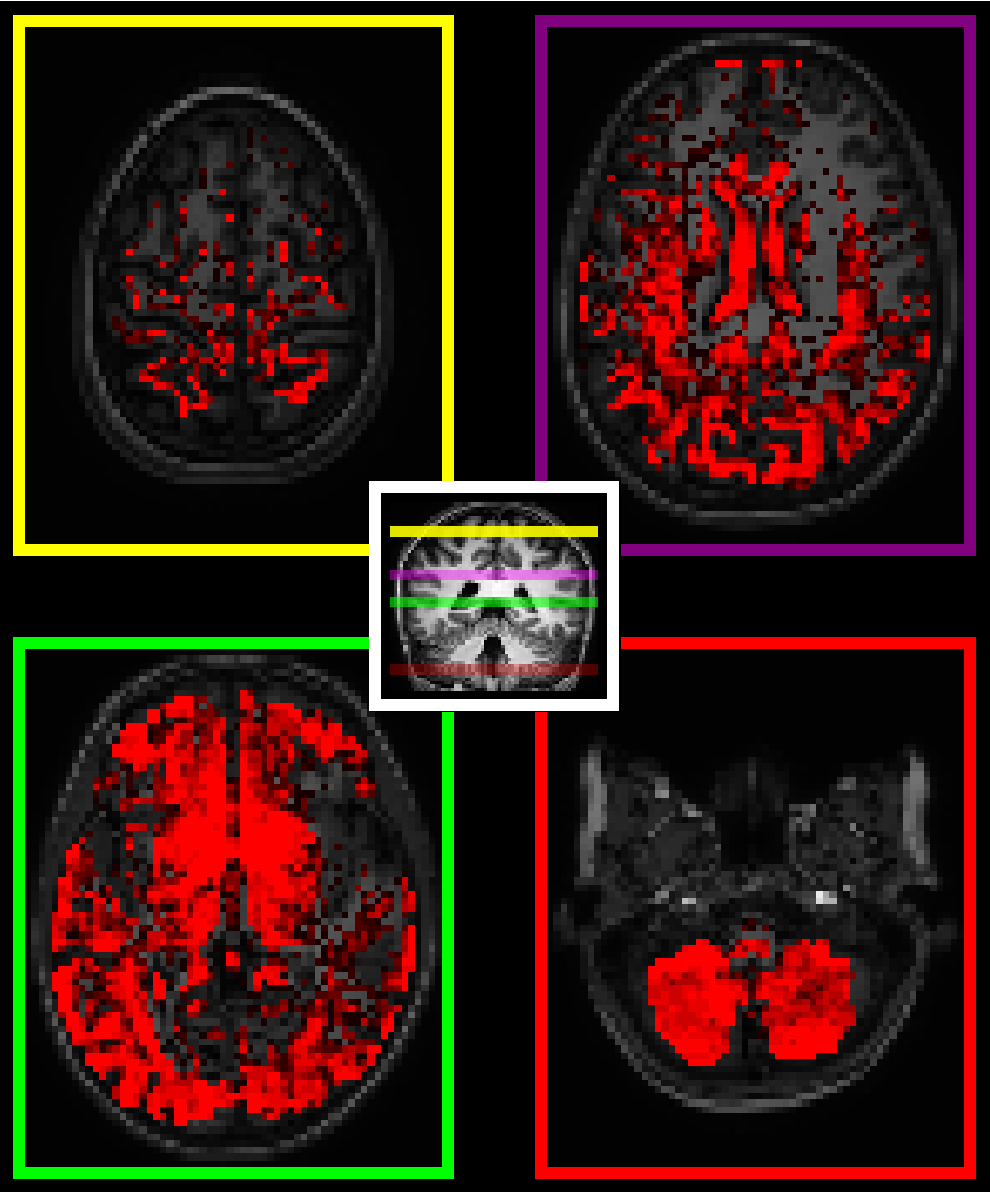
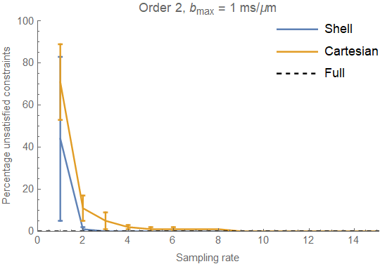
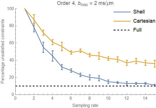
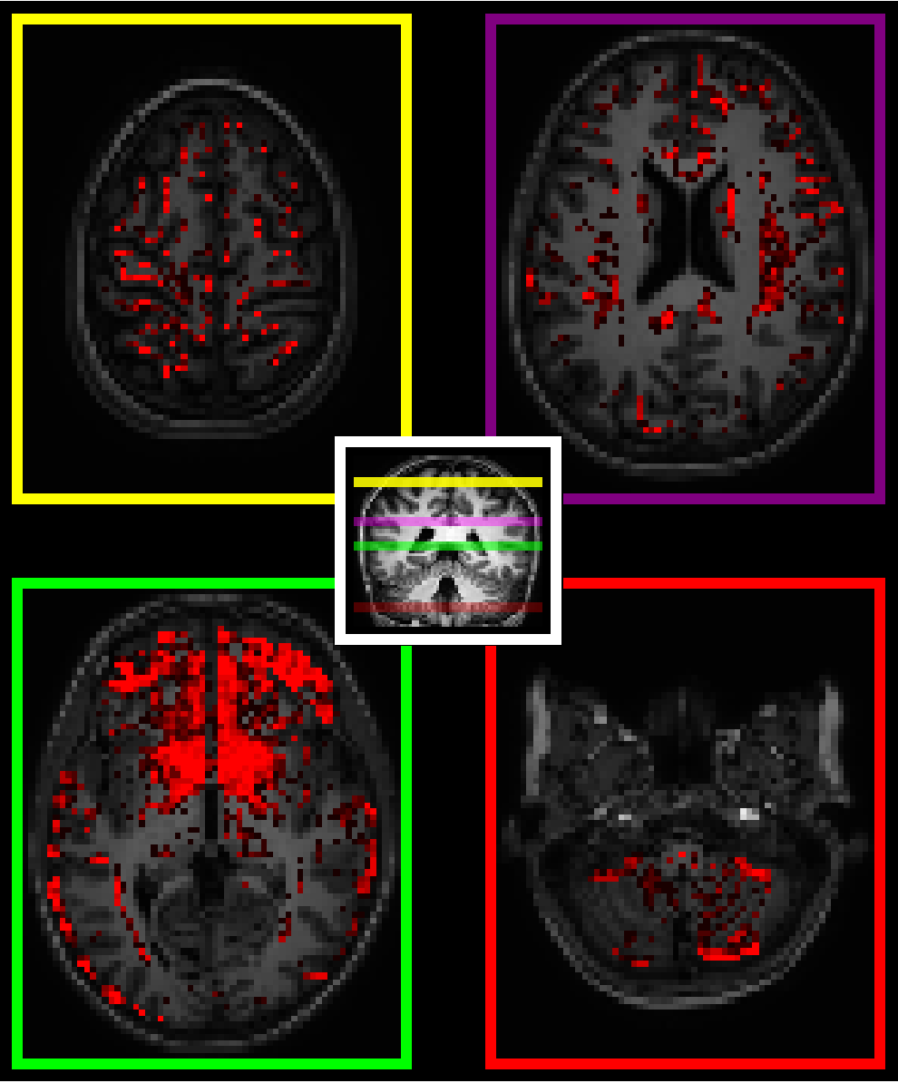
In Figs. 1 and 2 we plot the percentage of voxels in the brain where the constraints are not satisfied, with each data point computed as the mean number of 'incorrect' voxels in $$$10$$$ randomly sub-sampled data sets. The dashed black line indicates the percentage of incorrect voxels obtained when using all available measurements (suitable for a given order). Voxels where the constraints are not satisfied appear to be concentrated near the interface between white and gray matter and in deep structures in all cases (ignoring masking errors), as can be seen in Figs. 3 and 4. In the case of space-filling sampling the ventricles also contain a large number of invalid voxels.
Discussion
As expected, we observe a decreasing trend when increasing the sampling rate, and it turns out that this decrease is significantly more rapid in the case of spherical sampling. We note that spherical sampling works better in white matter and cerebro-spinal fluid, while space-filling sampling may have a (slight) edge around white matter-gray matter boundaries.
Secondly we note that when computing cumulants of orders greater than two, it is quite essential to take the considered constraints into account during reconstruction—despite the fact that a constrained least squares reconstruction increases the computation time from several minutes to several hours. This becomes even more apparent when we include $$$b$$$-values up to $$$3 \, \textrm{ms}/\mu\textrm{m}^2$$$ and compute cumulants up to order six, in which case over half ($$$51\%$$$) of the voxels fail to satisfy the necessary constraints even with a (practically infeasible) best-case sampling rate of $$$\sim 60$$$, and in this case we may even conclude that we need better quality data or higher $$$b$$$-values to obtain a reliable reconstruction.
Although alternatives to the cumulant expansion may be more resilient, it seems likely that a constrained reconstruction could also be beneficial in many of those cases. In future work we will investigate the necessity and practicality of convex-constrained reconstruction in other models.
Acknowledgements
The authors gratefully acknowledge the Villum Foundation for financial support.References
[1] Tom Dela Haije et al. "Reconstruction of convex polynomial di ffusion MRI models using semi-de finite programming". In: Proceedings of the 23rd Annual Meeting of the ISMRM. 2015, p. 2821.
[2] Martijn Froeling et al. "MASSIVE brain dataset: Multiple acquisitions for standardization of structural imaging validation and evaluation". In: Magnetic Resonance in Medicine (2016).
[3] Jelle Veraart et al. "Constrained maximum likelihood estimation of the diff usion kurtosis tensor using a Rician noise model". In: Magnetic Resonance in Medicine 66.3 (2011), pp. 678-686.
[4] Makoto Yamashita et al. A high-performance software package for semidefi nite programs: SDPA 7. Research Report B-460.Tokyo Institute of Technology, 2010.
Figures
Spatial localization of voxels with unsatisfied constraints in the case of shell-based sampling, with a sampling rate of $$$15$$$; brightness of the red voxels indicates the fraction of the $$$10$$$ randomly sub-sampled data sets that produced invalid voxels at that location. A T1-weighted image is shown in the background for anatomical reference. Voxels with unsatisfied constraints appear to be concentrated at the white matter-gray matter interface and in deep structures, with some small regions of consistently invalid voxels appearing in white matter bundles.