Synopsis

We studied the orientationally averaged diffusion weighted MR signal for diffusion along general curves at all three temporal regimes of the traditional pulsed field gradient measurements. We found that long fibers as well as short fibers that are straight could yield the $$$q^{-1}$$$ decay. The absence of such a decay suggests fibers that are short and curvy. We note that the true asymptotic behavior of the signal decay is characterized by the Debye-Porod law, which suggests $$$\bar{E}(q)\propto q^{-4}$$$ at very large $$$q$$$-values. This study is expected to provide insights for interpreting the diffusion-weighted images of the central nervous system.

Introduction

Upon averaging the three-dimensional q-space MR signal over respective shells in q-space, a one-dimensional signal attenuation profile, $$$\bar E(q)$$$, is obtained. $$$\bar E(q)$$$ represents the decay for the “powdered” specimen, which contains an isotropic distribution of each and every compartment in the original specimen.

In a recent study [1], such orientationally averaged signal was reported to exhibit the power-law $$$\bar E(q)\propto q^{-1}$$$ in white-matter and a distinctively faster decay in gray-matter was observed. Since neuronal and glial projections can be envisioned to be tubes of infinitesimal diameter [2] as far as diffusion measurements via clinical scanners are concerned, we studied the effects of curvilinear diffusion on the orientationally averaged signal.

Theory

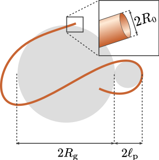
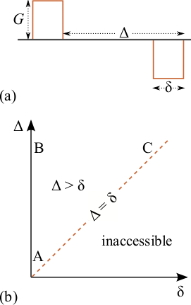
Figure 1 illustrates the relevant size parameters of a simplified neural projection, which can be described by a curve $$$\mathbf{r}(s)$$$ parameterized by its arclength $$$s$$$. We consider the Stejskal-Tanner measurement [3] whose effective gradient waveform is shown in Figure 2a. There are three distinct temporal regimes of this experiment depending on whether the timing parameters are short or long (see Figure 2b):

• Regime A: In this short diffusion time regime, each particle diffuses along a straight line segment.

• Regime B: This is the "scattering regime" realized by widely-separated narrow pulses. In this regime, every particle can diffuse to any point on the curve.

• Regime C: Very long pulses leads to a Gaussian signal.

At small q-values, the compartmental signal is well approximated by a Gaussian, i.e., $$$E (\mathbf{q})\approx e^{- \mathbf{q}^T \mathbf{V} \mathbf{q}}$$$, where $$$\mathbf{V}$$$ is the signal decay tensor, which is given in the three temporal regimes by the following expressions:

$$ V^A_{ij}=\frac{D \Delta}{\ell} \int_0^\ell \mathrm{d}s \, \frac{\mathrm{d} r_i(s)}{\mathrm{d} s} \frac{\mathrm{d} r_j(s)}{\mathrm{d} s} $$

$$ V^B_{ij}= \frac 1\ell \int_0^\ell \mathrm{d} s \, R_i(s) \, R_j (s)$$

$$ V^C_{ij}= \frac{2}{D \delta} \int_0^\ell \mathrm{d} s \, r_i(s) \int_0^\ell \mathrm{d} s' \, r_j(s') \left\{ B_2\left( \frac{|s-s'|}{2\ell} \right) + B_2\left( \frac{s+s'}{2\ell} \right) + \frac{\ell^2}{3 D \delta} \left[ B_4\left( \frac{|s-s'|}{2\ell} \right) + B_4\left( \frac{s+s'}{2\ell} \right) \right] \right\} $$

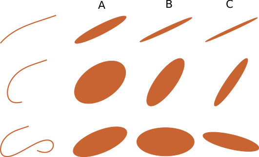
where $$$D$$$ is the bulk diffusivity, $$$\mathbf{R}(s)$$$ represents the curve in a frame of reference whose origin coincides with the center-of-mass of the curve, and $$$B_n(\cdot )$$$ denotes the $n$th order Bernoulli polynomial. The signal decay tensors for three representative curves are depicted in Figure 3.

At intermediate q-values, the orientationally averaged signal profiles were found to be

$$ \bar E^A(q) = \frac{\sqrt{\pi}\, \mathrm{erf}(q\sqrt{D\Delta})}{2q\sqrt{D\Delta}} $$

$$ \bar E^B(q) = \frac{1}{\ell^2} \int_0^\ell \mathrm{d}s \int_0^\ell \mathrm{d} s' \, \frac{\sin \left[ q \, |\mathbf r(s) - \mathbf r(s')| \right]}{q \, |\mathbf r(s) - \mathbf r(s')|} $$

$$ \bar E^C(q) = \frac{\sqrt{\pi}\, e^{- q^2 v_\perp} \mathrm{erf}(q\sqrt{v_\parallel - v_\perp})}{2q\sqrt{v_\parallel -v_\perp}} $$

where $$$v_\parallel$$$ and $$$v_\perp$$$ indicate the eigenvalues of the signal decay tensor (assuming axial symmetry).

Finally, at very large-q ($$$q R_0 \gg 1$$$): Debye-Porod law [4], $$$\bar E(q)\propto q^{-4}$$$, applies.

Discussion

The above findings can be discussed separately for the three temporal regimes of the experiment. In regime C, the compartmental signal is Gaussian and the orientationally-averaged signal exhibits $$$q^{-1}$$$ behavior only when the signal decay tensor is rank-1, i.e., for straight fibers. In regimes A and B, however, the $$$q^{-1}$$$ behavior is not a consequence of the signal decay tensor having rank 1. In regime A, it is the dominant behavior beyond a crossover value $$$q \sqrt{D\Delta} \approx 1$$$. Regime B shares the same math with small angle scattering experiments employed for characterizing the structure of polymers [5]. For example, wormlike structures are characterized by a decay $$$\propto q^{-1}$$$ at $$$q$$$-values about the reciprocal of the chain's persistence length. Thus, even non-straight structures exhibit $$$q^{-1}$$$ decay in Regime B even though the signal decay tensor is not of rank 1.

In light of our study, the findings in [1] can be interpreted as follows: In white-matter, there appears to be a substantial presence of long fibers that could be straight or curved and/or short fibers that are straight. The opposite appears to be true for gray-matter in which the fibers would have to be shorter and curved. Indeed, gray-matter is rich in dendrites and unmyelinated axons, which will exhibit a fair amount of bending distributed across any voxel.

Conclusion

Acknowledgements

References

1. McKinnon ET, Jensen JH, Glenn GR, et al. Dependence on b-value of the direction-averaged diffusion-weighted imaging signal in brain. Magn Reson Imaging. 2017;36:121–127.

2. Kroenke CD, Ackerman JJH, Yablonskiy DA. On the nature of the NAA diffusion attenuated MR signal in the central nervous system. Magn Reson Med. 2004;52:1052–1059.

3. Stejskal EO, Tanner JE. Spin diffusion measurements: Spin echoes in the presence of a time-dependent field gradient. J Chem Phys. 1965;42:288–292.

4. Sen PN, Hürlimann MD, de Swiet TM. Debye-Porod law of diffraction for diffusion in porous media. Phys Rev B. 1995;51:601–604.

5. Glatter O, Kratky O, eds. Small Angle X-Ray Scattering. 1982;London: Academic Press.