Synopsis

In this study, we combined complex network theory with machine learning in order to grasp potential biomarkers of brain development. The data consists of brain connectomes (brain connectivity matrices) of 53 children aged six years old. For each subject, we estimated brain network-based measures at four different levels: connection, node, module and global levels. Then we applied linear discriminant analysis and support vector machine in order to extract features and we compared their performances. We showed that node and module levels are the best choices to extract relevant and interpretable biomarkers in order to distinguish between different brain development conditions.

Introduction

Methods

Subjects

The data consists of brain connectomes of 53 children aged six years old, provided by the Child Developmental Unit at the University Hospitals of Geneva and Lausanne2. Children were grouped in three different classes: 9 were born moderate preterm with normal birth weight and considered as moderate preterm (MP); 21 subjects were born moderately preterm with intra uterine growth restriction (IUGR); 23 were born at <28 weeks of gestational age and considered as extreme premature (EP).

Acquisition

For each subject, T1-weighted MPRAGE images (TR/TE=2500/2.91, TI=1100, res.=1x1x1mm, 256x154) and diffusion-weighted images, using a diffusion-sensitized EPI sequence (30 directions, max b-value=1000 s/mm2, TR/TE=10200/107, res=1.8x1.8x2 mm), were acquired on a 3T Tim Trio system.

Preprocessing

For each subject, we extracted a symmetric connectivity matrix using the connectome map toolkit3. Each connectivity matrix (or brain network) was defined on the basis of 83 regions of interests (ROIs) or nodes and the value of the connectivity between each pair of nodes reflects the mean fractional anisotropy (FA) value of the bundle connecting each pair of cortical regions.

Analysis

The aim of the study is to show how we can extract network-based features in order to distinguish between the three groups (MP, IUGR and EP). To achieve this, we used brain network-based measures at four different levels.

Connection level: We used all connection values as features (the upper triangle of the connectivity matrix) resulting in 1829 features per subject.

Node level: We considered three integration/segregation nodal topological measures: nodal strength, nodal clustering and nodal efficiency4 for each node resulting in 249 (3x83) features per subject.

Module level: We decomposed the average MP network that we considered as control group and by applying different modularity maximization based algorithms5. We averaged the three nodal features across each community for each subject resulting in number of features per subject equal to three times the number of communities. The algorithms yield different numbers of communities. However, the number of features is less than the half of the number of subjects in all cases.

Global level: We averaged the three nodal features across all nodes, resulting in three features per subject.

After normalizing all features, we performed linear discriminant analysis (LDA) to features estimated at both global and module levels since the number of features is less the number of subjects at these two levels, whereas Support Vector Machine was applied at connection and node levels. We assessed the accuracy of the LDA and SVM for each case. To avoid over-fitting, we used leave-one-out cross-validation.

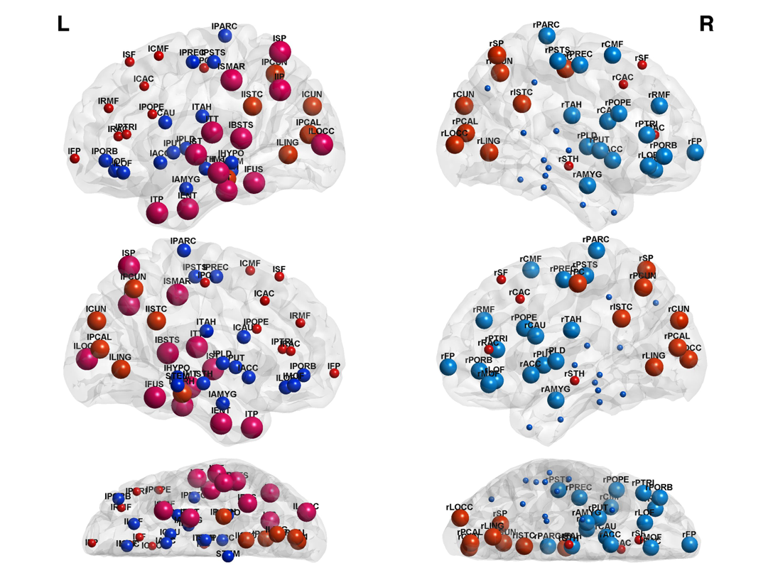
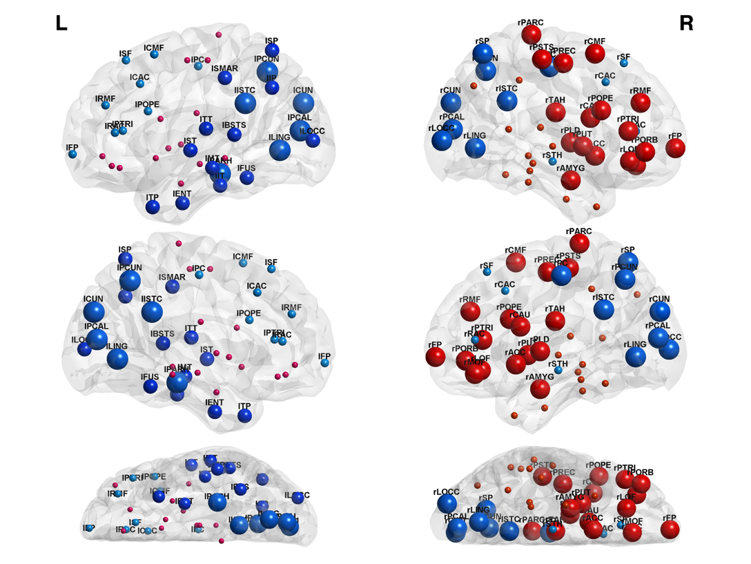
Finally, we represented LDA projection at the module level with Leading Eigen Vector (LEV) decomposition in the form of brain maps.

Results and Discussion

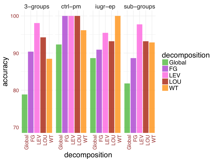
Fig. 1 shows the LDA accuracy at both global and modular levels. Interestingly, considering local features increases tremendously the classification accuracy, which reaches very high levels in some cases. Potentially, this indicates that differences among the 3-groups are more localized rather than global differences, which is in line with the hypothesis that EP and IUGR represent two different conditions affecting different brain regions and connections6.

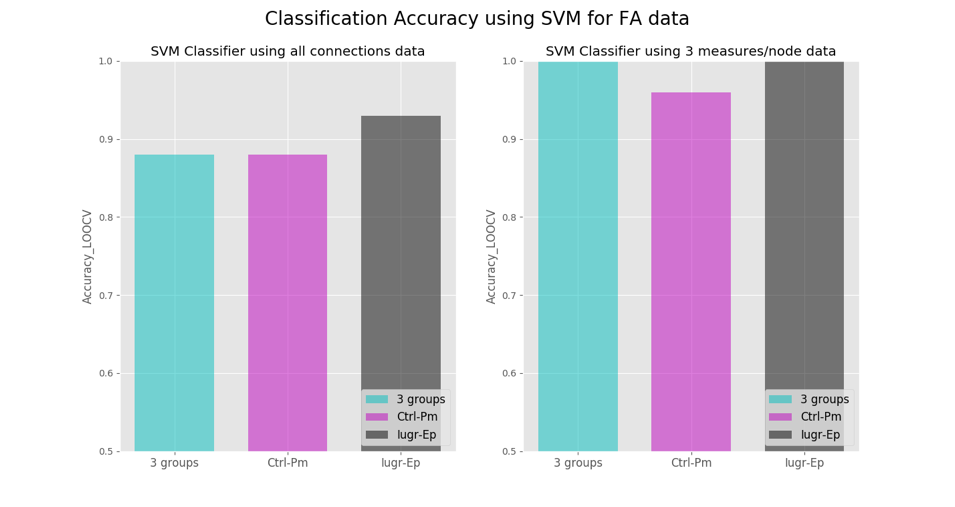
Furthermore, by observing Fig. 2, we can see that because nodal measures incorporate more complex data structure information, give better accuracy compared to connection based SVM. Finally, from Fig. 3 and Fig. 4 we identify the biomarker as the contrast in strength and efficiency between different brain modules.

Conclusions

Acknowledgements

References

1. Fischi-Gomez, E. et al. Brain network characterization of high-risk preterm-born school-age children. NeuroImage Clin. 11, 195–209 (2016).

2. Meskaldji, D. E. et al. Improved statistical evaluation of group differences in connectomes by screening-filtering strategy with application to study maturation of brain connections between childhood and adolescence. Neuroimage 108, 251–264 (2015).

3. Connectome Map Toolkit: http://www.cmtk.org. Accessed on November 01,2017.

4. Fischi-Gómez, E. et al. Structural Brain Connectivity in School-Age Preterm Infants Provides Evidence for Impaired Networks Relevant for Higher Order Cognitive Skills and Social Cognition. Cereb. Cortex 25, 2793–2805 (2015).

5. Meskaldji, D. E. et al. Comparing connectomes across subjects and populations at different scales. Neuroimage 80, 416–425 (2013).

6. Meskaldji, D. E. et al. Adaptive strategy for the statistical analysis of connectomes. PLoS One 6, (2011).