5113
Accelerating 3D CEST Imaging with Low Rank Sparse Reconstruction1Radiology, UT Southwestern Medical Center, Dallas, TX, United States, 2Philips Research, Hamburg, Germany, 3Advanced Imaging Research Center, UT Southwestern Medical Center, Dallas, TX, United States, 4Philips Healthcare, Gainesville, FL, United States
Synopsis
Chemical exchange saturation transfer (CEST) is a new contrast mechanism in MRI. However, a successful application of CEST is hampered by its slow acquisition especially in the 3D applications. Compressed sensing (CS) is powerful for reconstruction of highly undersampled data. This work implements the 3D pulsed steady-state CEST acquisition sequence and extended the low rank plus sparse (L+S) method to a 3D version. The phantom and in vivo human brain results demonstrate our design has the potential to accelerate the 3D CEST imaging about 4 times.
Purpose
Chemical exchange saturation transfer (CEST) is a new contrast mechanism that can indirectly visualize the low concentration metabolites, which are not observable in conventional MR scans. [1]. However, CEST acquisition can be time-consuming and ways to speed-up the acquisition are desired. Compressed sensing (CS) [2,3] techniques have been used to accelerate 2D CEST imaging [4-6]. However, the biggest contributor to the long acquisition time in 2D CEST is actually the saturation pulse. The real advantages of CS reconstructions would be in the expansion of the methods to 3D CEST [7-9]. In this study we implement a 3D pulsed steady-state CEST acquisition sequence [8] and propose a 3D low rank plus sparse (L+S) method [10] for 3D reconstruction. The phantom and in vivo human brain experiments show that this CS scheme may accelerate 3D CEST acquisition by factor of R = 4.Acquisition Method
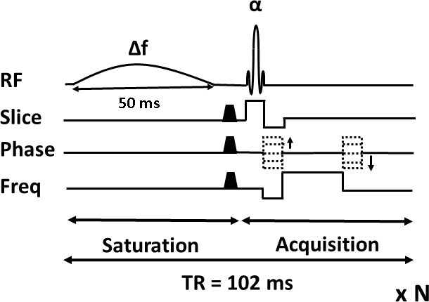
All experiments were performed on a Philips 3T MRI scanner using a 32 channel head coil. 3D pulsed steady-state CEST pulse sequence [8] was implemented as shown in Figure 1. The saturation block consisted of a frequency-selective saturation pulse of 50 ms duration followed by crusher gradients (0.5 ms duration and 10 mT/m strength). Saturation block was applied before an acquisition block of the same duration and was employed before the acquisition of each k-space line. 3D B0 map is acquired with the standard protocol for B0 inhomogeneity correction. The acquisition parameters for the phantom and brain data are described below.
Phantom: The phantom consists of five tubes of Iopamidol solution with pH values of 6.0, 6.5, 7.0, 7.5, and 8.0. The Sinc-Gaussian pulse was used for saturation (pulse duration=50 ms, flip angle=900°, and B1rms = 2.69 μT). Phantom data was acquired with the following parameters: flip angle α = 10°, TR/TE = 102/2.2 ms, FOV=192x192x24 mm3, resolution=2x2x0.75 mm3, matrix=96x96x32. 11 saturation frequencies were acquired swept between ±1000 Hz in steps of 200 Hz. A separate reference scan was acquired with an off-resonance frequency of 400 kHz. The total acquisition time was 48 minutes.
Human brain: Human brain data was acquired with similar parameters as phantom, except we have used Hyperbolic-Secant pulse, B1rms=1.51 μT, TR/TE=102/1.6 ms, FOV=220x220x40 mm3, resolution = 2.5x2.5x5 mm3, matrix = 96x96x8. The total acquisition time was 9 minutes.
Reconstruction Method
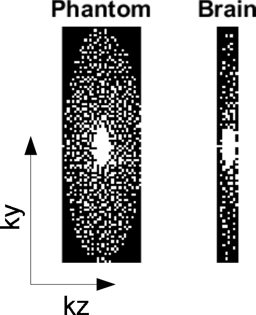
In CEST imaging, voxels in the same compartment have similar Z-spectra [4]. The high spatiotemporal correlation is suitable for the low rank matrix model. We extended the L+S [10] method into a 3D version to address the additional sparse prior information in the z-dimension, based on the assumption that the pixels at adjacent slices have high correlations. The extended 3D L+S decompose the 3D CEST spatial-temporal matrix as a summation of a low-rank matrix (few non-zero singular values) and a sparse matrix (few non-zero elements). Specifically, the reconstruction algorithm tries to solve this problem: $$$min_{L,S} ||F(L+S)-d||^2_2+λ||L||_*+η||S||_1$$$, where $$$F$$$ is the undersampling Fourier operator, $$$d$$$ is the undersampled k-space data, $$$||\cdot||_*$$$ is the nuclear norm to regularize the sparsity of the low-rank matrix $$$L$$$, $$$||\cdot||_1$$$ is the L1-norm to regularize the sparsity of the sparse matrix $$$S$$$, $$$λ$$$ and $$$η$$$ are regularization parameters. Before reconstruction, the data is normalized to make the mean value equals to 1, then the regularization parameters are robust to both phantom and brain data. We select parameters as $$$λ=0.002$$$ and $$$η=0.01$$$. Poisson-disc undersampling pattern [11] of reduction factor R=4 was used to evaluate the algorithm (Figure 2).Results
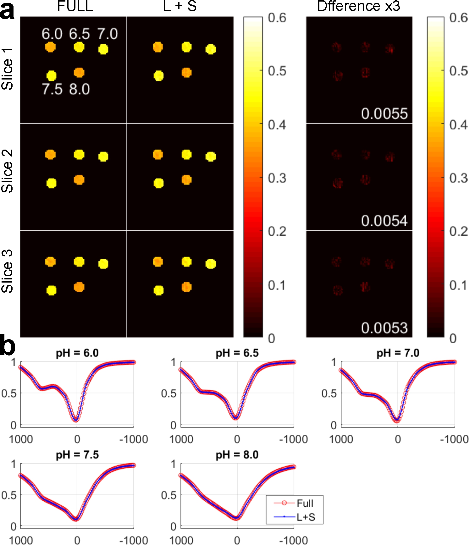
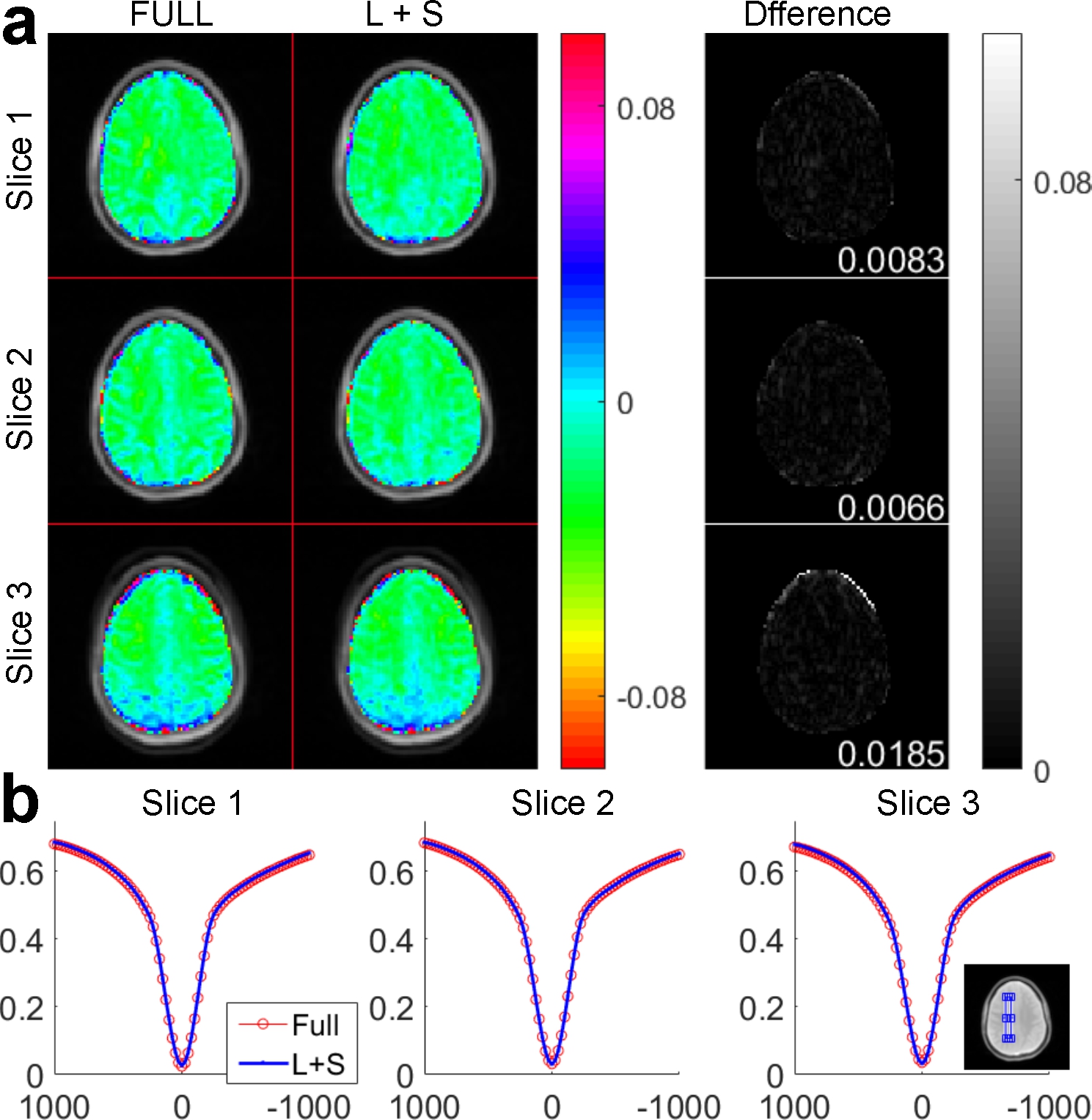
Figure 3 compares MTRasym (4.2ppm) map and Z-spectra between the reconstruction of fully sampled and undersampled phantom data. Three slices are shown for evaluation. From the normalized root mean square error (nRMSE) of the L+S reconstruction shown at the bottom right corner of the Difference images, the reconstructed MTRasym maps are close to the fully sampled ones. The Z-spectra of L+S reconstruction are also close to the fully sampled ones for five different pH values. Figure 4 demonstrates the MTRasym (3.5ppm) maps and averaged Z-spectra in the region of interest for the brain. Three slices are shown for evaluation. The reconstructed MTRasym maps and Z-spectra are also similar to the fully sampled ones.Conclusion
We propose and test a 3D version of the low rank plus sparse (L+S) method. The phantom and in vivo human brain results demonstrate that our design has the potential to accelerate the 3D CEST imaging about 4 times. Work is underway to experimentally test accelerating in vivo 3D CEST imaging using the undersampling pattern and reconstruction algorithm described in this study.Acknowledgements
The authors thank Dr. Ricardo Otazo (New York University) for making the low rank plus sparse matrix decomposition (L+S) code available online. The authors thank Dr. Asghar Hajibeigi (University of Texas Southwestern Medical Center) for phantom preparation. This work was supported by the NIH grant R21 EB020245 and by the UTSW Radiology Research fund.References
[1] van Zijl P, et al. MRM 2011;65:927–948.
[2] Candes EJ, et al. IEEE TIT 2006;52:489–509.
[3] Donoho DL. IEEE TIT 2006;52:1289–1306.
[4] Zhang Y, et al. MRM 2016;76:136–144.
[5] Heo HY, et al. MRM 2017;77:779–786.
[6] She H, et al. ISMRM 2016;2904.
[7] Zhu H, et al. MRM 2010;64:638–644.
[8] Jones CK, et.al. MRM 2012;67:1579–1589.
[9] Zhang Y, et al. ISMRM 2017;1971.
[10] Otazo R, et al. MRM 2015;73:1125-36.
[11] Lustig M, et al. ISMRM 2009;379.
Figures