Purpose

Chemical exchange saturation transfer (CEST) is a novel and promising contrast mechanism in MRI [1]. However, a successful translation of CEST into clinic might be hampered by its time-consuming acquisition. Parallel imaging methods such as SENSE [2] are widely used to accelerating MRI. However, SENSE is limited in CEST by reconstruction accuracy [3]. Convolutional Neural Networks (CNN) is a deep learning method for MRI reconstruction [4-7], which trains a neural network to connect the undersampled images with the fully sampled images. Cascade-CNN [7] learns a mapping from undersampled images to the fully sampled images with a cascade network layers, and shows high quality reconstruction for the test data in the single coil case. However, it did not consider the case of multi-channel MRI imaging, which is the standard method in MRI scan. We extended the Cascade-CNN into a parallel-CNN (PCNN) network combining multi-coil data to accelerate CEST. The proposed method shows good reconstruction quality for in vivo brain CEST data at acceleration factor R=4.

Theory

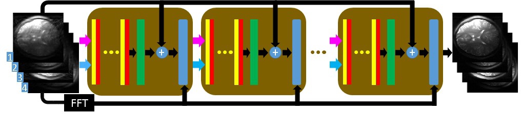
In the extended version of CNN developed and tested here, the PCNN, the input of the CNN is composed of multi-coil undersampled images, and the output of the CNN is composed of multi-coil fully sampled images. PCNN can learn the mapping of multi-coil data similar to SENSE [2]. As shown in Fig. 1, after extracting the real part (purple arrows) and imaginary part (blue arrows) from the input data, the multi-channel data is fed into the network. The network is cascaded by several blocks (brown squares) [7] to improve reconstruction quality. Each block includes several convolutional layers (yellow bars) followed by activation layers (red bars), fully connect layer (green bars), residual layer (summations), and data consistency (DC) layer (blue bars). The residual layer can help the network converge faster [8]. The DC layer can constraint the reconstruction image to be consistent to the fully sampled k-space data [7].

Methods

All the experiments were performed on a Philips 3T scanner using a 32-channel head coil. All CEST images were acquired with a TSE sequence, TR/TE=4200/6.4 ms, slice thickness=4.4mm, matrix=240x240, FOV=240x240mm². The saturation RF consisted of 40 Hyperbolic Secant or Sinc-Gaussian pulses each of 49.5 ms duration with 0.5 ms intervals; 31 offset points were swept between ±1000Hz in steps of 67Hz with one additional image acquired without saturation for normalization. Three saturation power levels were tested: 0.7 μT, 1.2 μT, and 1.6 μT. Ten sets of in vivo human brain data were collected for training, and the other two datasets for testing. CEST processing used WASSR [9] for B₀ inhomogeneity correction. Data augmentation was used for the training data to avoid the overfitting problem. The MTR_asym­ maps were calculated at 3.5 ppm (amide proton transfer). PCNN was implemented with Python. All the computations were performed on a Lenovo workstation with Intel Xeon CPU and NVidia GeForce GPU. Since the reconstruction using 32 channels data took too much GPU memory, the software channel compression [10] was performed to combine the 32-coil data into 4 virtual coils. Currently, we have evaluated the performance of PCNN by performing retrospective Cartesian undersampling [11], and the acceleration factor was R=4. Evaluations at higher acceleration factors (R=6,8,etc) are underway.

Results

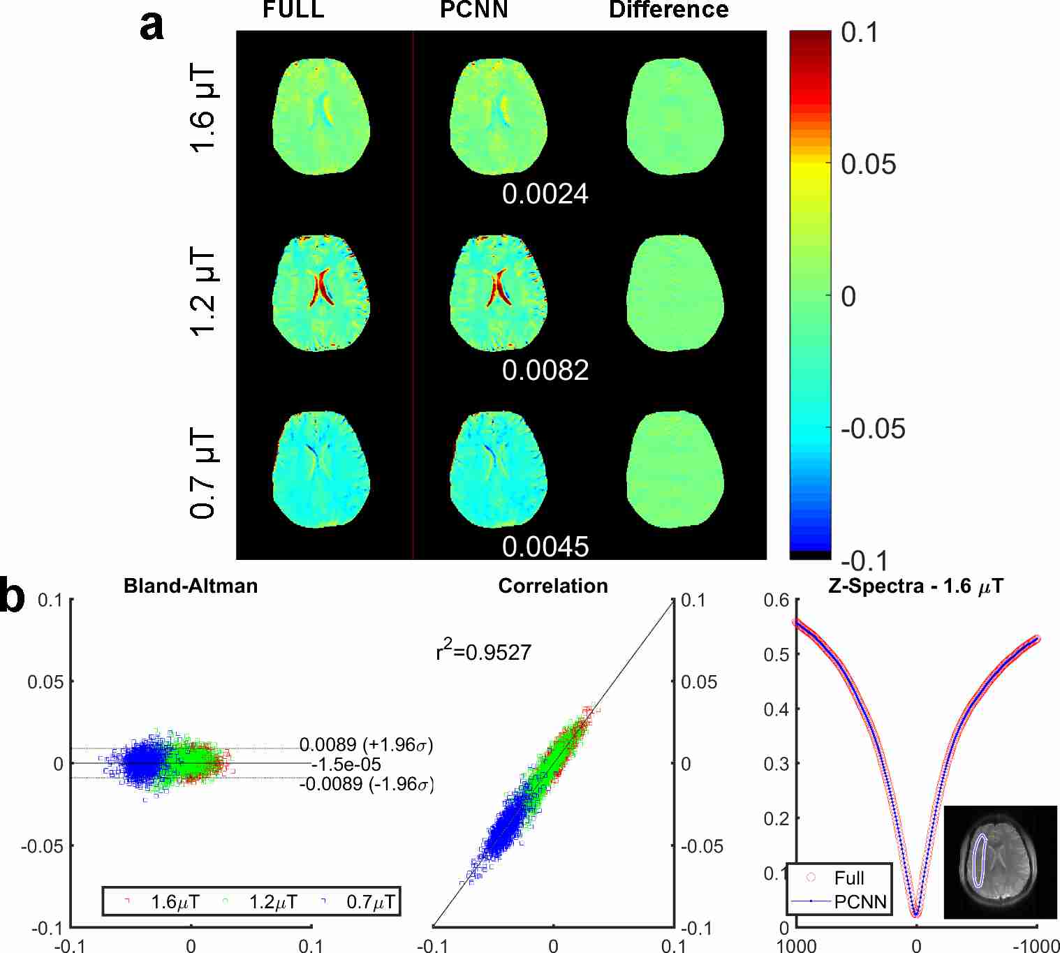
Fig. 2 compares the results reconstructed with fully sampled and PCNN for an in vivo brain dataset using an Hyperbolic Secant saturation pulse at different saturation power levels. In Fig. 2(a), the reconstruction MTR_asym maps and difference images demonstrate that PCNN can give high reconstruction quality similar to the fully sampled case. Fig. 2 (b) shows the Bland-Altman plot [12] and correlation plot reconstructed with PCNN and the fully sampled case for different saturation power in the region of interest (ROI). The ROI is shown at the bottom right corner. It is evident that PCNN leads to a high correlation with the fully sampled data. Fig. 2 (b) also shows that PCNN gives similar ROI-averaged Z-spectrum to fully sampled data. Fig. 3 shows the results of another dataset with Sinc-Gaussian saturation pulses, and the conclusion is the same and it shows that PCNN can also give high reconstruction quality at different saturation pulses.

Conclusion

We propose a parallel convolutional neural networks (PCNN) method for CEST imaging. In vivo human brain results demonstrate that the proposed method is able to reconstruct the image similar to fully sampled case at reduction factor of R=4. Work is in progress to collect more training dataset at different saturation time and evaluate the method in larger populations of volunteers.

Acknowledgements

The authors thank Mr. Jo Schlemper and Dr. Jose Caballero (Imperial College London) for making the Cascade-CNN code available online. The authors thank Dr. Asghar Hajibeigi (University of Texas Southwestern Medical Center) for phantom preparation. This work was supported by the NIH grant R21 EB020245 and by the UTSW Radiology Research fund.