Purpose

Chemical exchange saturation transfer (CEST) is a new contrast mechanism with many promising applications [1]. However, the translation of CEST into clinical is hampered in part by its long acquisition times. Compressed sensing (CS) [2-5] provides a way to accelerate the MRI acquisition, by utilizing the sparse information embedded in the data. Previously we and other groups applied Blind CS (BCS) to CEST [6-8]. However, there are other CS reconstruction methods that may provide more acceleration or better contrast and resolution fidelity. Patch-based dictionary learning method is different and well-known CS method, which tries to find sparse coding in the data [9]. However, the original method only considers the sparsity in local patch, but does not consider the global sparsity in the CEST data. To accelerate CEST, here we propose a patch-based global orthogonal dictionary learning method, named G-KSVD method, which leads to high quality reconstruction at a high reduction factor R=8.

Theory

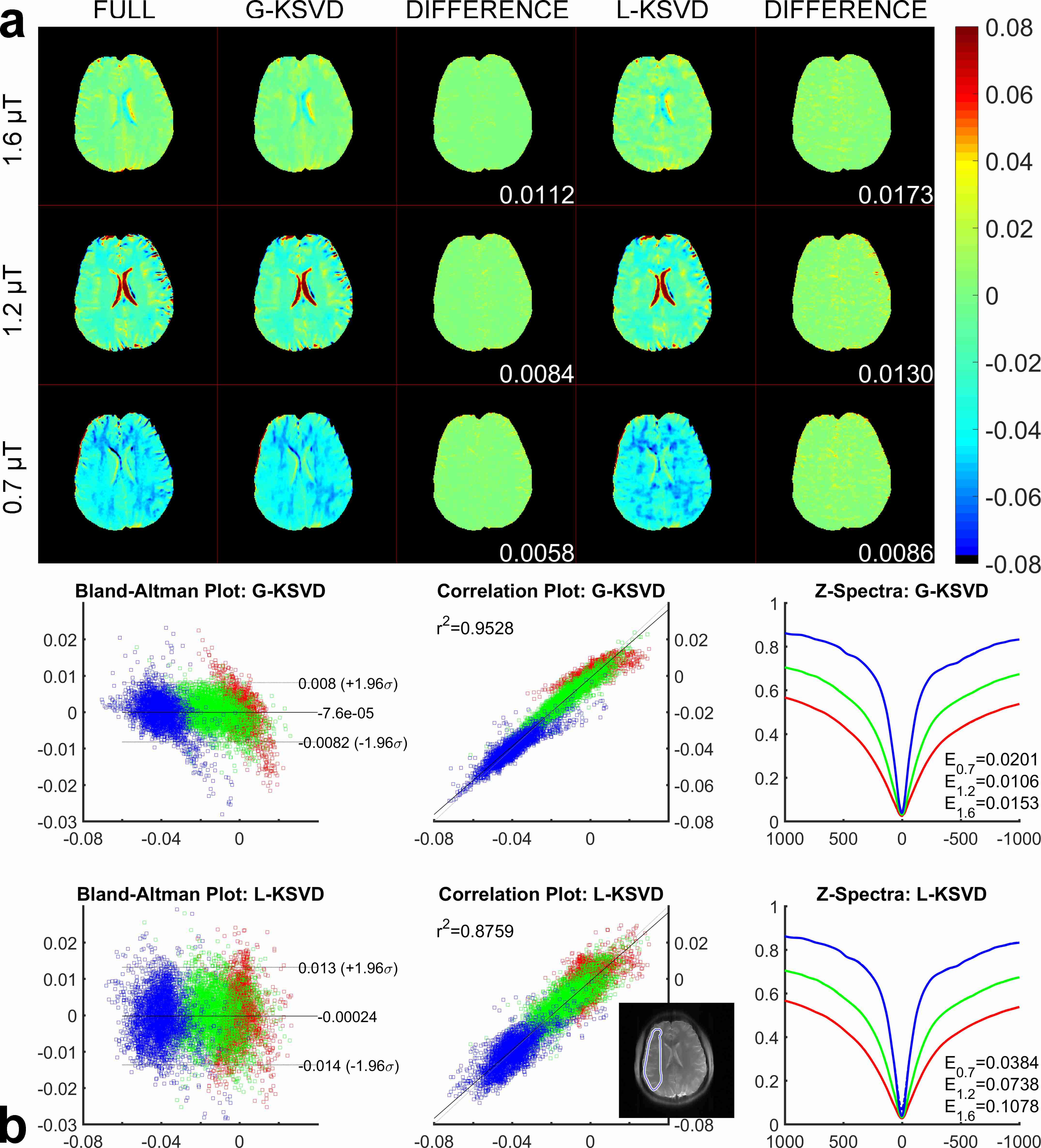
In traditional local patch-based dictionary learning L-KSVD [9], the image series is divided into small local patches along $$$x-y-t$$$ dimension. L-KSVD only utilized the local information in the temporal domain due to the small patch size in the $$$t$$$ dimension. As we know, CEST data has high spatial-temporal correlation, i.e. the Z-spectrum in local spatial domain shows high similarity in global temporal domain. Thus, the global temporal information in CEST data might not been grasped by the traditional sparse dictionary representation. For G-KSVD, the images are divided into global patches along $$$t$$$ dimension and local patches along $$$x-y$$$ dimensions. In this way, G-KSVD not only grasp the local image sparsity in spatial domain, but also grasp the global sparsity in temporal domain. Specifically, G-KSVD tries to solve the following problem: $$$min_{x,D,γ_i} ∑_i ||F_ux-y||^2_2+α||P_ix-Dγ_i||^2_2, s.t. ||γ_i||_0<ε, ∀i$$$, where $$$x$$$ is the desired CEST dynamic images, $$$F_u$$$ is the undersampled Fourier operator, $$$y$$$ is the undersampled k-space data, $$$P_ix$$$ extracts the $$$i$$$-th cubic patch from $$$x$$$, $$$γ_i$$$ is the sparse coefficient of the $$$i$$$-th patch using the dictionary $$$D$$$, $$$||\cdot||_0$$$ is the $$$L_0$$$ norm, $$$ε$$$ is the threshold of the sparsity, $$$α$$$ is the regularization parameter.

Methods

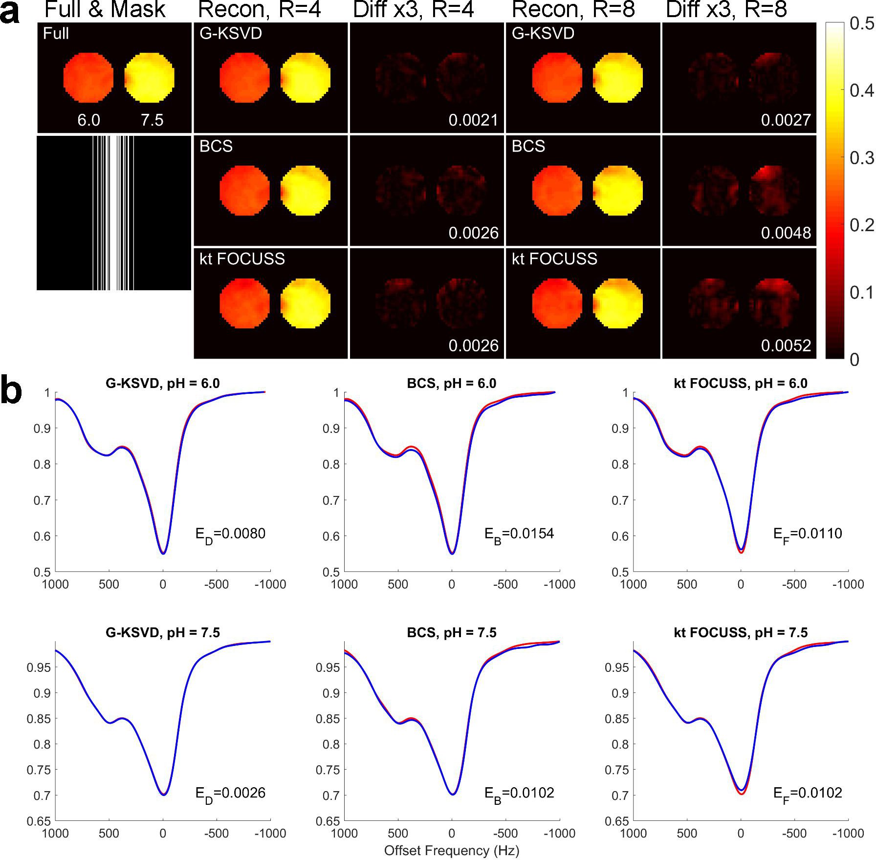
The phantom consists of two tubes of Iopamidol solution with pH values of 6.0 and 7.5. In vivo human brain data from n=2 volunteers was also collected. All images were acquired on a Philips 3T scanner using a 32-channel head coil and a TSE sequence with parameters: TR/TE=4200/6.4 ms, slice thickness=4.4 mm, matrix=240x240, FOV=240x240 mm. The saturation RF consisted of 40 pulses each of 49.5 ms duration with 0.5 ms interval; 31 offset points were swept between ±1000 Hz in steps of 67 Hz. One additional image was acquired without saturation for normalization. The saturation power is 1.6 μT, 1.2 μT, 0.7 μT. CEST processing used WASSR [10] for B₀ inhomogeneity correction. The MTR_asym­ maps were calculated at 4.2 ppm for phantom, and 3.5 ppm (amide proton transfer) for brain. We used the variable density Cartesian random undersampling pattern to retrospectively sample the data [3].

Results and Discussion

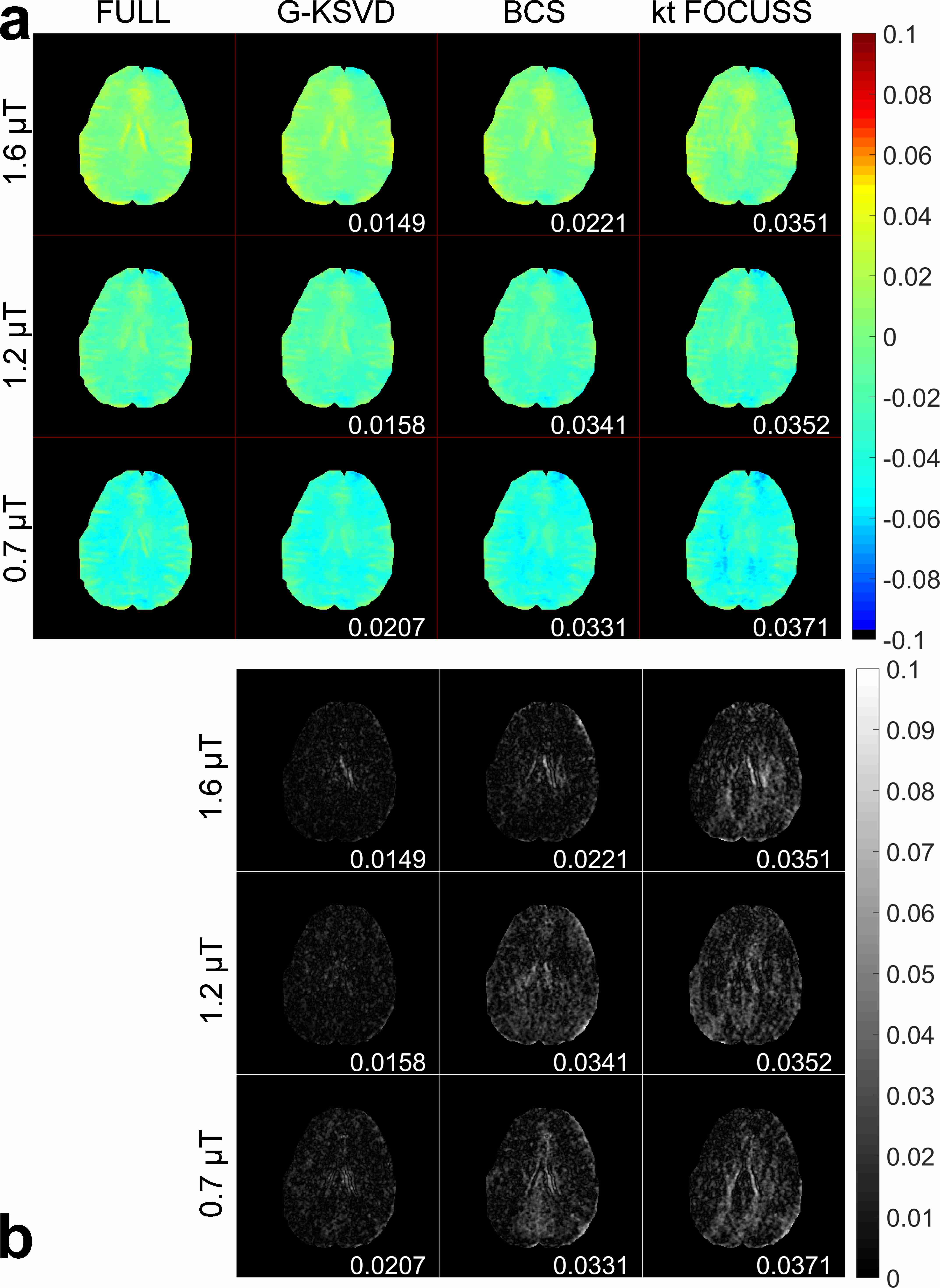
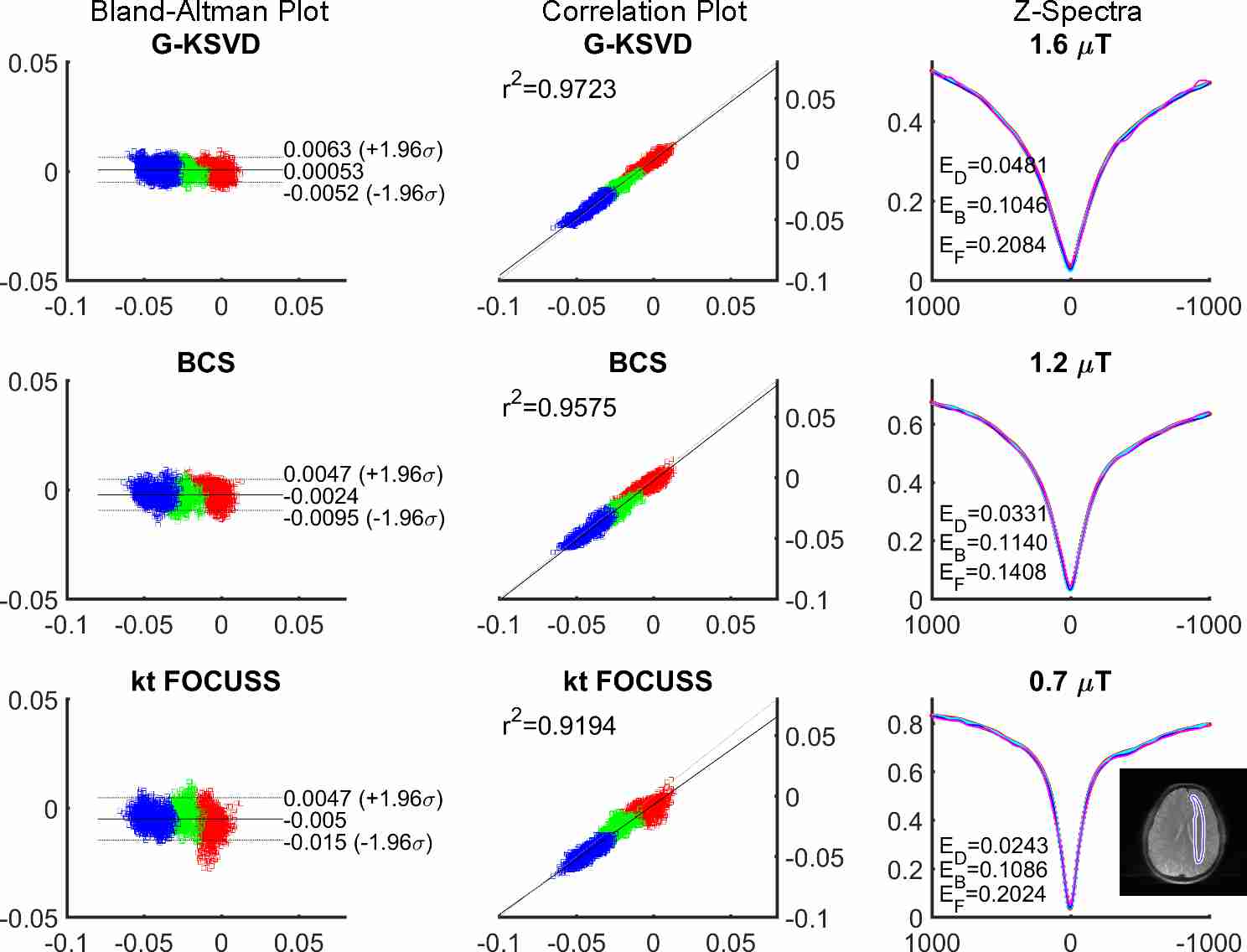
Fig. 1 compares MTR_asym and Z-spectra with fully sampled, G-KSVD, BCS [4] and k-t FOCUSS [5] for phantom. G-KSVD gives a smaller root mean square error (nRMSE) at reduction factors R=4 and 8. In Fig 2 (a-b), in-vivo MTR_asym map using G-KSVD is superior to BCS and k-t FOCUSS in that it has less aliasing and errors. In Fig. 3, G-KSVD method with R = 8 generates similar Z-spectra, compared to the fully sampled case, while k-t FOCUSS deviates from the fully sampled case at some frequency ranges. The nRMSE of the reconstructed Z-spectra of G-KSVD (E_D), BCS (E_B), and k-t FOCUSS (E_F) are shown, and G-KSVD has the smallest reconstruction error. To address the advantage of the proposed global patch-based G-KSVD we compare it with L-KSVD. As shown in Fig. 4, the reconstruction results of L-KSVD is not as good as the proposed G-KSVD method. G-KSVD has smaller reconstruction aliasing in the MTR_asym map, and smaller standard deviation in the Bland-Altman plot, and better $$$r^2$$$ value in the correlation plot. For Z-spectra, L-KSVD deviates at the zero-frequency part, but G-KSVD is closer to the fully sampled case. The nRMSE values of reconstructed Z-spectra of G-KSVD and L-KSVD at different saturation powers, 0.7 μT (E_0.7), 1.2 μT (E_1.2), and 1.6 μT (E_1.6) are also shown.

Conclusion

We proposed a G-KSVD method to accelerate CEST imaging. Phantom and in vivo results demonstrate that the proposed method is capable of providing more accurate reconstructions at high reduction factors compared with BCS and k-t FOCUSS.

Acknowledgements

The authors thank Dr. Jose Caballero (Imperial College London) for making the dictionary learning (DLTG) code available online. The authors thank Dr. Asghar Hajibeigi (University of Texas Southwestern Medical Center) for phantom preparation. This work was supported by the NIH grant R21 EB020245 and by the UTSW Radiology Research fund.