Synopsis

Electrical properties tomography (EPT) is a promising technique that has the potential to generate high resolution images of tissue electrical properties in vivo. One limitation of EPT is its high sensitivity to noise in the measured data. In this study, a comparison was performed between the so-called gradient-based EPT (gEPT) algorithm and the Helmholtz-based EPT method in a simulation. The result suggests significantly improved performance using gEPT and provides useful insight into the noise behavior of various EPT algorithms for optimization of the algorithm design.

Introduction

Methods

Simulation

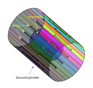
A 16-rung TEM coil and a cylindrical phantom was modeled as shown in Fig. 1. The TEM coil has a ground shield with 64.8 cm in diameter and 100 cm in length. Each rung is 41.2 cm in length and 2.4cm in width, consisting of three 13.2 cm long, capacitor-connected strips. The coil is tuned to 127.75 MHz equivalent to the resonance frequency at 3 T. The phantom model is 30cm in diameter and 41.8cm in length, of which uniform EPs are set to $$$\sigma=0.59S/m$$$ and $$$\varepsilon=73.6\varepsilon_0$$$ for grey matter (GM) or $$$\sigma=0.34S/m$$$ and $$$\varepsilon=52.6\varepsilon_0$$$ for white matter (WM). Here, $$$\varepsilon_0$$$ is the permittivity of free space. The simulation was conducted based on the finite-difference time-domain method in Sim4Life (Zurich Med Tech), and a 1 mm isotropic mesh is applied to the model. Each rung was excited one after another by a voltage source at one end of the strip.

EPT Reconstruction

The relationship between EPs and the transmit ($$$B_1^+$$$) and receive ($$$B_1^-$$$) $$$B_1$$$ field is[9]:\begin{align*}-\nabla^2B_1^+&=\omega^2\varepsilon_c\mu_0B_1^+-\Big(\frac{\partial{B_1^+}}{\partial x}-i\frac{\partial{B_1^+}}{\partial{y}}\Big)(g_x+ig_y)-\frac{\partial{B_1^+}}{\partial{z}}g_z\qquad&(1)\\-\nabla^2B_1^{-*}&=\omega^2\varepsilon_c\mu_0B_1^{-*}-\Big(\frac{\partial{B_1^{-*}}}{\partial{x}}+i\frac{\partial{B_1^{-*}}}{\partial{y}}\Big)(g_x-ig_y)-\frac{\partial{B_1^{-*}}}{\partial{z}}g_z\qquad &(2)\end{align*}where $$$\varepsilon_c:=\varepsilon-i\frac{\sigma}{\omega}$$$ is the complex permittivity, $$$(g_x,g_y,g_z):=\nabla\ln\varepsilon_c$$$ the gradient of the logarithm of $$$\varepsilon_c$$$, $$$\mu_0$$$the magnetic permeability of free space and $$$\omega$$$ the angular resonant frequency. Both gETP reconstruction (GR) and Helmholtz-based reconstruction (HR) were performed using the simulated $$$B_1$$$ data. Using GR, sixteen channels of $$$B_1^+$$$ and $$$B_1^-$$$ were used for calculating $$$g_x$$$, $$$g_y$$$ and $$$g_z$$$ in (1) and (2); the EP distribution was calculated from $$$g_x$$$ and $$$g_y$$$ in 2D slices using the finite-difference method with known EP value on a single seed point at the center of the model [3]. Using HR, EPs are calculated directly in Eqs.(1) and (2) using the same $$$B_1^+$$$ and $$$B_1^-$$$ data, with $$$g_x$$$, $$$g_y$$$ and $$$g_z$$$ set to zero. Reconstruction was performed within a region of interest (ROI) of $$$100\times100\times20mm^3$$$ at the center of the phantom. For GR, various in-plane sizes of the ROI were further utilized to evaluate its effect on SNR of the reconstructed EPs (SNREP).

Before reconstruction, Gaussian noise was added to the B1 data with a standard deviation (SD) equal to 1/SNR_B1 of the mean magnitude of $$$B_1$$$ within the ROI ( $$$100\times100\times20mm^3$$$). A 3D low-pass Gaussian filter with a SD of $$$\sigma_f$$$and kernel size, which is in voxels equivalent to six times of $$$\sigma_f$$$, was utilized to smooth the noise-contaminated $$$B_1$$$ data. To estimate the variance of the reconstructed EPs, a bootstrap strategy with 10 counts was performed for each set of parameters. SNREP was calculated as the ratio between the target EPs and the mean variance of the reconstructed EPs.

Results

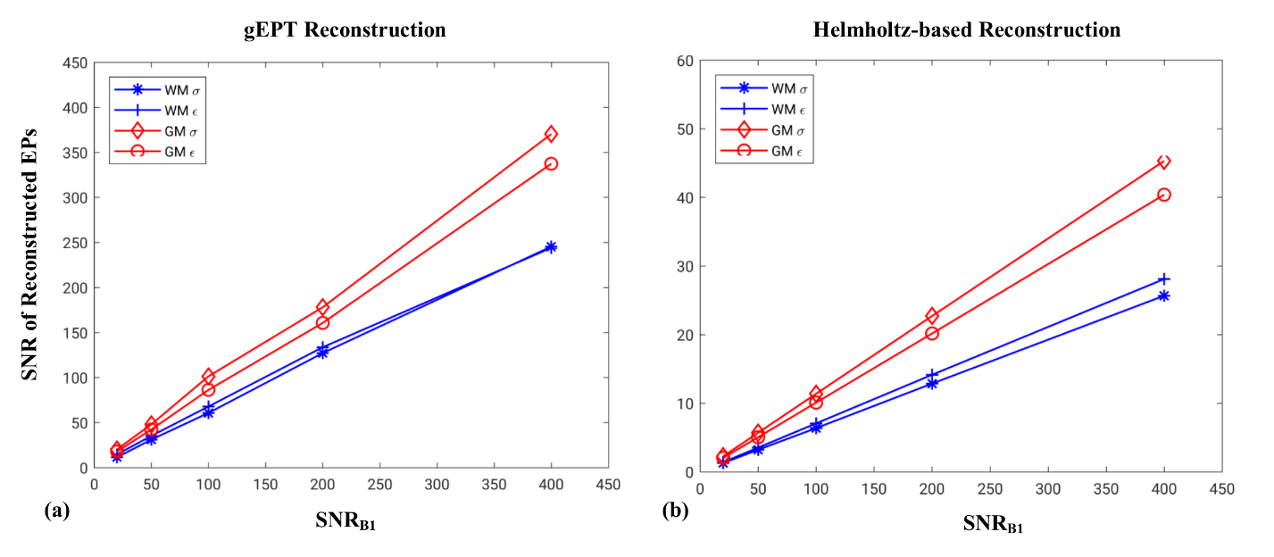
Relationship between SNR_EP and SNR_B1 is shown in Fig. 2a and 2b for GR and HR ($$$\sigma_f=1.8 mm$$$), respectively. As can be observed, SNR_EP of GR is close to 10 times that of HR. Using GR, a small non-linearity is observed at low SNR_B1 in comparison with that of HR.

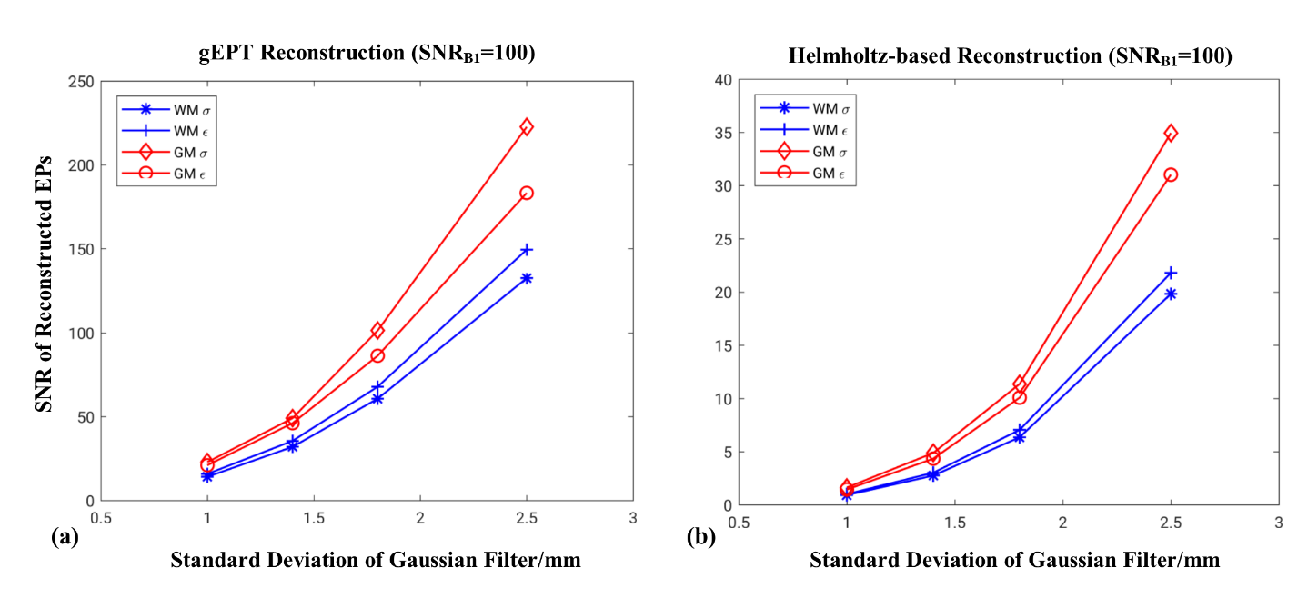
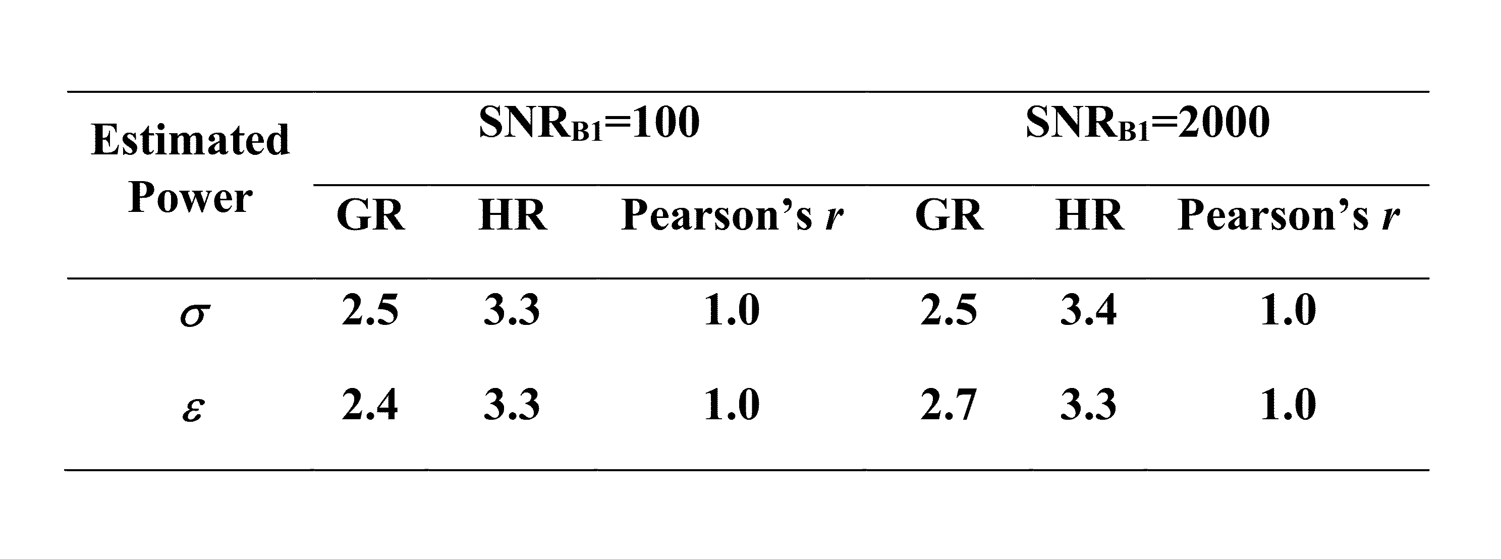
With various $$$\sigma_f$$$, the impact of low-pass filter or equivalently the effective resolution of the $$$B_1$$$ data is investigated and results shown in Fig. 3. Previous analysis suggested SNR_EP$$$ \propto \sigma_f^{3.5}$$$ using a 3D filter[7]. Here, regression analysis on the results of GM shows a power value of ~3.3 for HR and ~2.5 for GR with Pearson’s $$$r$$$ values close to 1 (Tab.1). The slightly lower power of the HR relationship (3.3 vs. theoretical 3.5) could be due to the non-uniform $$$B_1$$$ magnitude of individual TEM coils.

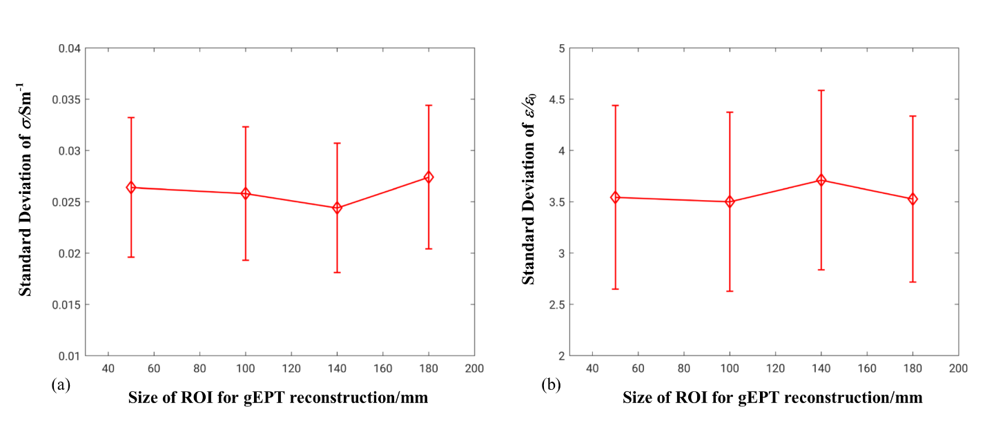
The effect of in-plane ROI size on the robustness of GR is shown in Fig. 4 based on the GM model. The result doesn’t suggest a significant impact on the variance of EPs due to different ROI sizes.

Discussion

Acknowledgements

References

[1] U. Katscher, T. Voigt, C. Findeklee, P. Vernickel, K. Nehrke, and O. Dossel, “Determination of Electric Conductivity and Local SAR Via B1 Mapping,” IEEE Trans. Med. Imag., vol. 28, no. 9, pp. 1365–1374, Sep. 2009.

[2] X. Zhang, S. Zhu, and B. He, “Imaging Electric Properties of Biological Tissues by RF Field Mapping in MRI,” IEEE Trans. Med. Imaging, vol. 29, no. 2, pp. 474–481, Feb. 2010.

[3] J. Liu, X. Zhang, S. Schmitter, P.-F. Van de Moortele, and B. He, “Gradient-based electrical properties tomography (gEPT): A robust method for mapping electrical properties of biological tissues in vivo using magnetic resonance imaging,” Magn. Reson. Med., vol. 74, no. 3, pp. 634–646, Sep. 2015.

[4] S.-K. Lee, S. Bulumulla, F. Wiesinger, L. Sacolick, W. Sun, and I. Hancu, “Tissue electrical property mapping from zero echo-time magnetic resonance imaging,” IEEE Trans. Med. Imaging, vol. 34, no. 2, pp. 541–550, Feb. 2015.

[5] F. S. Hafalir, O. F. Oran, N. Gurler, and Y. Z. Ider, “Convection-reaction equation based magnetic resonance electrical properties tomography (cr-MREPT),” IEEE Trans. Med. Imaging, vol. 33, no. 3, pp. 777–793, Mar. 2014.

[6] E. Balidemaj et al., “CSI-EPT: A Contrast Source Inversion Approach for Improved MRI-Based Electric Properties Tomography,” IEEE Trans. Med. Imaging, vol. 34, no. 9, pp. 1788–1796, Sep. 2015.

[7] S.-K. Lee, S. Bulumulla, and I. Hancu, “Theoretical Investigation of Random Noise-Limited Signal-to-Noise Ratio in MR-Based Electrical Properties Tomography,” IEEE Trans. Med. Imaging, vol. 34, no. 11, pp. 2220–2232, Nov. 2015.

[8] D. Sodickson et al., “Generalized Local Maxwell Tomography for Mapping of Electrical Property Gradients and Tensors,” in Proceedings of the 21th Annual Meeting of ISMRM, Salt Lake City, USA, 2013, p. 4175.

[9] J. Liu, Y. Wang, U. Katscher, and B. He, “Electrical Properties Tomography Based on $B_{{1}}$ Maps in MRI: Principles, Applications, and Challenges,” IEEE Trans. Biomed. Eng., vol. 64, no. 11, pp. 2515–2530, Nov. 2017.