5099
A Dictionary-Based Method for Conductivity Tensor Mapping1Biomedical Engineering, University of Michigan, Ann Arbor, MI, United States, 2Functional MRI Laboratory, University of Michigan, Ann Arbor, MI, United States
Synopsis
Measuring conductivity tensors provides an additional layer of information as to how tissues in the body conduct electric current. Tissues with anisotropic conductivity values may include white matter tracts and muscle. Measurement of the tensor requires the object to rotate with respect to the main magnetic field of the MRI scanner, but the degree of rotation is severely limited in human subjects. We propose a dictionary-based approach that provides an estimate of the tensor given small rotation angles of the object.
Introduction
Conductivity mapping has applications in clinical diagnostics as well as RF safety. Measuring conductivity as a tensor provides additional information as to how tissues conduct electric current. The most common way to estimate the conductivity tensor is by scaling the diffusion tensor1. This assumes electric current is spatially restricted in the same manner as diffusion, which may not be true. There have been attempts at measuring the degree of anisotropy of electrical properties using MR electrical property tomography (MR-EPT)2,3, but to measure the tensor one must change the orientation of the object within the main magnetic field. This is challenging due to bore size and limited subject mobility. We propose a dictionary-based method for conductivity tensor mapping that allows for small degrees of rotation of the object within the bore.Theory
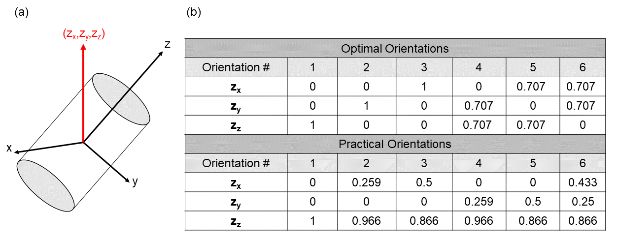
Let an object in a MRI scanner, which is allowed to rotate, have an object coordinate system, $$$(x,y,z)$$$, separate from the scanner coordinates, $$$(x',y',z')$$$. In some initial orientation the coordinate systems are the same, but as we rotate the object, the object coordinates are considered stationary while the scanner coordinates rotate. The following derivations assume that, because we can only measure the transverse component of the magnetic field in an MRI scanner, only the longitudinal component of the corresponding electric field is relevant to the problem. Thus, we define $$$\hat{z}=[z_x,z_y,z_z]$$$ as the unit vector in the direction of $$$\bf{B}_0$$$, with its components defined in terms of the object coordinate system, as shown in Figure 1a.
MR-EPT is derived from the homogeneous Helmholtz equation:
$$-\nabla^2\bf{H}=\nabla\times\it{j}\omega\kappa\bf{E}$$
$$\kappa = \frac{-\nabla^2\bf{H}}{\omega^2\mu_0\bf{H}}$$
where $$$\omega$$$ is the MRI resonant frequency and $$$\kappa=\epsilon-j\frac{\sigma}{\omega}$$$ is the complex permittivity, with $$$\epsilon$$$ the permittivity and $$$\sigma$$$ the conductivity. If $$$\kappa$$$ is anisotropic, its apparent value will depend on the orientation of the object.
The tensor $$$\underline{\underline{\kappa}}$$$ is symmetric and can be written as:
$$\underline{\underline{\kappa}}=\it\begin{bmatrix}\kappa_1&\kappa_4&\kappa_6\\\kappa_4&\kappa_2&\kappa_5\\\kappa_6&\kappa_5&\kappa_3\end{bmatrix}; \underline{\kappa}=\begin{bmatrix}\kappa_1&\kappa_2&\kappa_3&\kappa_4&\kappa_5&\kappa_6\end{bmatrix}$$
At a given orientation we measure the magnetic field, $$$\bf\tilde{H}$$$, and calculate the apparent value of $$$\kappa$$$. First, we examine how $$$\bf\tilde{H}$$$ changes with object orientation. We define the orientation-dependent electric field in terms of the field $$$\bf{E}=\tt[\it{{E}}_{x'},{{E}}_{y'},{{E}}_{z'}\tt]$$$, whose components are in scanner coordinates,
$$\bf\tilde{{E}}=\underline{\underline{\kappa}}{E}=\it\underline{\underline{\kappa}}\tt[\it{{E}}_{x'},{{E}}_{y'},{{E}}_{z'}\tt]$$
and assume $$$\bf{E}$$$ and $$$\underline{\underline{\kappa}}$$$ are constant. By Faraday's law, $$$\bf\tilde{H}$$$ is proportional to the curl of $$$\bf\tilde{E}$$$, but only the longitudinal component of $$$\bf\tilde{E}$$$ is relevant:
$$\bf\tilde{{E}}\cdot\it\hat{z}=\kappa_1E_{x'}z_x+\kappa_2E_{y'}z_y+\kappa_3E_{z'}z_z+\kappa_4E_{y'}z_x+\kappa_4E_{x'}z_y+\kappa_5E_{z'}z_y+\kappa_5E_{y'}z_z+\kappa_6E_{z'}z_x+\kappa_6E_{x'}z_z.$$
We also only consider the longitudinal component of $$$\bf{E}$$$, which is a scaled version of $$$\hat{z}$$$, so:
$$\bf\tilde{{E}}\cdot\it\hat{z}\propto\tt[\it\kappa_1z_xz_x,\kappa_2z_yz_y,\kappa_3z_zz_z,2\kappa_4z_xz_y,2\kappa_5z_yz_z,2\kappa_6z_xz_z\tt].$$
We define the vector
$$\bf{z}=\tt[\it{z_xz_x,z_yz_y,z_zz_z,2z_xz_y,2z_yz_z,2z_xz_z}\tt]$$
and describe the magnetic field as
$$\bf\tilde{{H}}\propto\underline{\kappa}\cdot\bf{z}\it=\begin{bmatrix}\kappa_1&\kappa_2&\kappa_3&\kappa_4&\kappa_5&\kappa_6\end{bmatrix}\cdot\tt[\it{z_xz_x,z_yz_y,z_zz_z,2z_xz_y,2z_yz_z,2z_xz_z}\tt].$$
To the leading order, the conductivity of a material primarily affects the phase of the magnetic field4. The phase-based conductivity approximation is
$$\sigma=\frac{\nabla^2\phi^+}{\omega\mu_0}$$
where $$$\phi^+$$$ is the phase of the transmit RF magnetic field. This approximation is linear and phase enters the receive coils linearly, so
$$\phi^+\propto\bf\underline{\Sigma}\cdot\bf{z}$$
where $$$\bf\underline{\Sigma}$$$ is the conductivity tensor.
If we measure the phase-based conductivity at six different orientations and concatenate them into a vector, $$$\bf{s}=\tt[\sigma_1,\sigma_2,\sigma_3,\sigma_4,\sigma_5,\sigma_6]$$$, we can solve for $$$\bf\underline{\Sigma}$$$ using the equation
$$\bf\underline{\Sigma}=\bf{Z^{-1}s}\tt.$$
Here, $$$\bf{Z}$$$ is size $$$6\times6$$$, where each column is the vector $$$\bf{z}$$$ corresponding to one orientation.
We also propose a dictionary-based method to calculate $$$\bf\underline{\Sigma}$$$. A dictionary of tensors is created and for every atom, $$$\bf\underline{\Sigma}_i$$$, we calculate the conductivity for each of the acquisition orientations,
$$\bf{s}_i=\underline{\Sigma}_i\bf{Z}.$$
The error is
$$error_i=||\bf{s}_i-s||,$$ and the optimal tensor is that with the lowest error.
Methods
Experiments were performed on a liquid phantom (σ=2.11 S/m) filled with drinking straws and a piece of beef shoulder. Images were acquired on a 3.0T GE scanner at the orientations listed in Figure 1b. The conductivity for each orientation was calculated using the phase-based approximation. In the straw phantom, the mean conductivity in each compartment at each orientation was used to compute a mean conductivity tensor. In the beef, the tensor was calculated pixel-wise. Conductivity tensors were calculated directly and with the dictionary approach. Diffusion tensors were also calculated from a 32 direction blip-up/blip-down scan using FSL5,6.Results
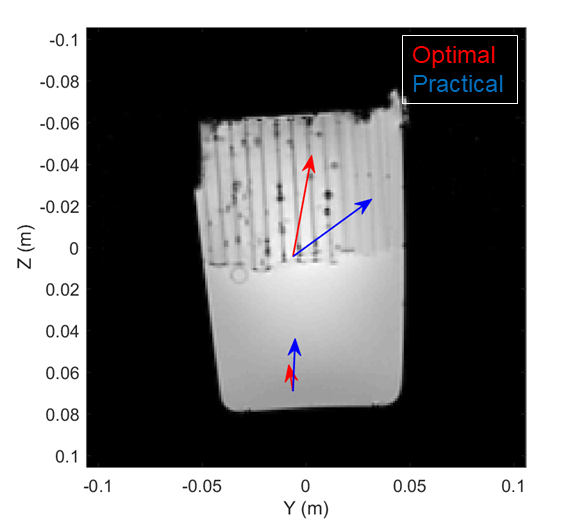
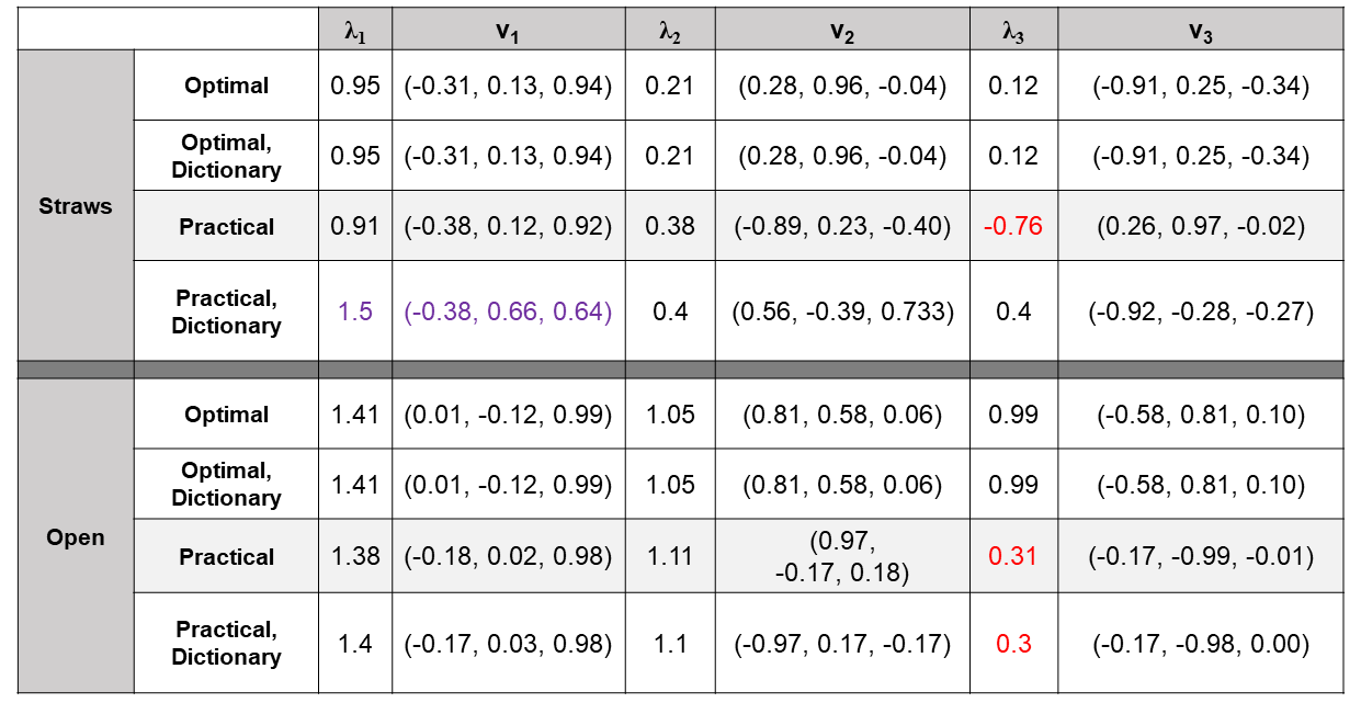
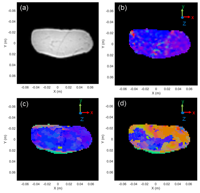
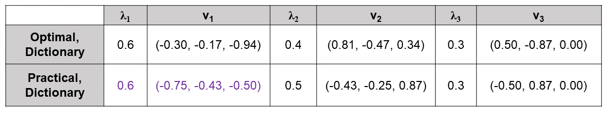
Figure 2 shows the mean conductivity tensor for Optimal Orientations aligns with the straws, but is biased for the Practical Orientations. Shown in Figure 3, using the dictionary approach with Practical Orientations yields all positive eigenvalues for the conductivity tensor, unlike with the direct calculation. Figures 4 and 5 show the conductivity and diffusion tensors in a slice of the beef. With Optimal Orientations, the conductivity and diffusion tensors are in agreement.
Discussion
Our proposed dictionary approach provides accurate tensor estimates for ideal object orientations. Given small, practical orientations, we are able to eliminate negative eigenvalues but there is a bias in the primary eigenvector. Conductivity tensors correlate well with the diffusion tensors, but conductivity may have anisotropic behavior on a larger scale than diffusion.
Acknowledgements
No acknowledgement found.References
[1] Tuch DS, Wedeen VJ, Dale AM, George JS, Belliveau JW. Conductivity tensor mapping of the human brain using diffusion tensor MRI. Proceedings of the National Academy of Sciences of the United States of America 2001;98:11697-11701.
[2] Katscher U, Voigt T, Findeklee C. Estimation of the Anisotropy of Electric Conductivity via B1 Mapping. Proceedings of the 18th Annual Meeting of the ISMRM 2010: 2866.
[3] Lee J, Song Y, Choi N, Cho S, Seo JK, Kim D-H. Noninvasive Measurement of Conductivity Anisotropy at Larmor Frequency Using MRI. Computational and Mathematical Methods in Medicine 2013: 421619.
[4] Wen H. Non-invasive quantitative mapping of conductivity and dielectric distributions using the RF wave propagation effects in high field MRI. In Proceedings of SPIE 5030, Medical Imaging 2003: Physics of Medical Imaging, San Diego, CA, USA, 2003: 471-477.
[5] Behrens TEJ, Woolrich MW, Jenkinson M, Johansen-Berg H, Nunes RG, Clare S, Matthews PM, Brady JM, Smith SM. Characterization and propagation of uncertainty in diffusion-weighted MR imaging. Magn Reson Med 2003;50:1077-1088.
[6] Jenkinson M, Beckmann CF, Behrens TE, Woolrich MW, Smith SM. FSL. NeuroImage 2012;62:782-90.
Figures