5098
Spatial resolution of Full cr-MREPT: 2D and 3D evaluation1Electrical and Electronics Engineering, Bilkent University, Ankara, Turkey
Synopsis
Determining the spatial resolution (SR) of Magnetic Resonance Electrical Property Tomography (MREPT) is important for assessing its utility in clinical applications. This study aims at finding the SR of Full cr-MREPT which yields images without internal boundary artifact. It is shown by simulations and experimental results that SR in general is determined by the resolution of the MR data. With noise-free simulation data SR is 2-2.5 pixels. With noisy and real data it may go up to 4-4.5 pixels due to Low Pass filtering and regularization. SR appears to be equal in all three directions.
Introduction
Convection-reaction equation based Magnetic Resonance Electrical Properties Tomography (cr-MREPT) aims at reconstructing EPs without internal boundary artifacts1,4. Spatial resolution (SR) is a measure of the ability to identify and separate high contrast small objects. High SR is important e.g. to delineate within-tumour conductivity variations or for brain imaging where small sulci and gyri dominate. Phase-based cr-MREPT has good SR but exhibits a global concave bias on conductivity values2,4. This study aims at studying SR of Full cr-MREPT1 which uses both the magnitude and the phase of $$$B_1^+$$$ and which is more accurate due to less stringent assumptions.Methods
Full crMREPT eliminates internal boundary artifacts by solving the equation $$$\beta\cdot\triangledown{u}+(\triangledown^2H^+)u-j\omega\mu_0H^+=0$$$ for $$$u$$$ which is the admittivity, $$$u=(\sigma+j\omega\epsilon)^{-1}$$$, and $$$\beta\cdot\triangledown{u}$$$ is the convection term with $$$\beta=\left[\frac{\partial{H^+}}{\partial{x}}-j\frac{\partial{H^+}}{\partial{y}}+\frac{1}{2}\frac{\partial{H_z}}{\partial{z}},{j}\frac{\partial{H^+}}{\partial{x}}+\frac{\partial{H^+}}{\partial{y}}+j\frac{1}{2}\frac{\partial{H_z}}{\partial{z}},\frac{\partial{H^+}}{\partial{z}}-\frac{1}{2}\frac{\partial{H_z}}{\partial{x}}-j\frac{1}{2}\frac{\partial{H_z}}{\partial{y}}\right]^T$$$.
For z-independent $$$u$$$ distributions the third row of the above PDE may be neglected and the problem reduces to 2D. Also in many cases, such as with birdcage volume excitation, the derivatives of $$$H_z$$$ are neglected1,7. The object is assumed to be composed of axial slices of equal distance between them in the z-direction. In case of a 2D application the Region of Interest (ROI) in a certain axial slice is discretized with a triangular mesh. For a 3D application the ROI selected on a certain slice is extended up and down for a specified number of axial slices. For regularization purposes a diffusion term $$$c_{diff}\triangledown^2u$$$ is added to the LHS where the diffusion constant $$$c_{diff}$$$ is experimentally found. Simulations are performed by COMSOL Multiphysics® (COMSOL AB, Sweden) where conductive objects are placed in a QBC coil6.
Results
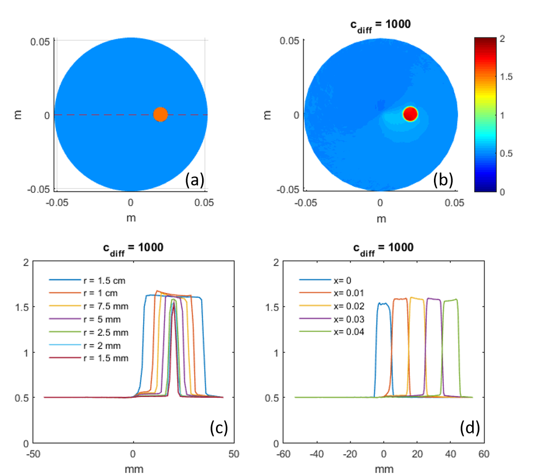
The capability of cr-MREPT to reconstruct conductivity of a single high contract object is shown in Figure-1. In this simulation there is no z-dependence of conductivity and therefore 2D cr-MREPT is used. Conductivity is reconstructed without boundary artifact and also accurately except for small objects (smaller than 3 mm radius). It also appears that reconstructions are not position dependent as the anomaly is moved from center to periphery.
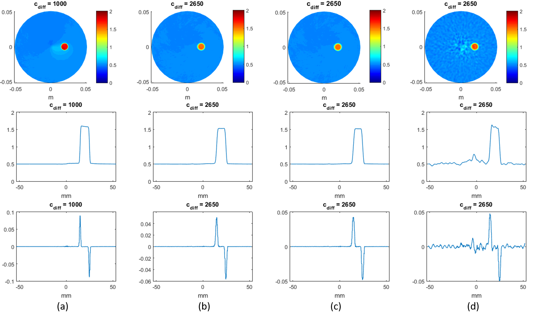
Point Spread Function (PSF) is obtained by taking the spatial derivative of the profiles shown in Figure-1 (see Figure-2). From the PSF, SR is calculated as the FWHM value and is found to be about 1.4 mm which is 2.3 times the pixxel size of 0.6 mm (Data are imported from Comsol environment on a Cartesian grid of 0.6mm voxel size in all directions). When a Gaussian 5x5 low pass filter with s.d. of 1.5 pixels or 3 pixels is used SR becomes 2 mm or 2.4 mm respectively. It is also found that an increase in $$$c_{diff}$$$ does not alter SR much except that it is useful to combat the so called "LCF artifact" especially when data are noisy1. In such case SR is the same but there is more irregularity in the center of the phantom where the Low Convective Field region is (region where $$$\beta$$$ is low).
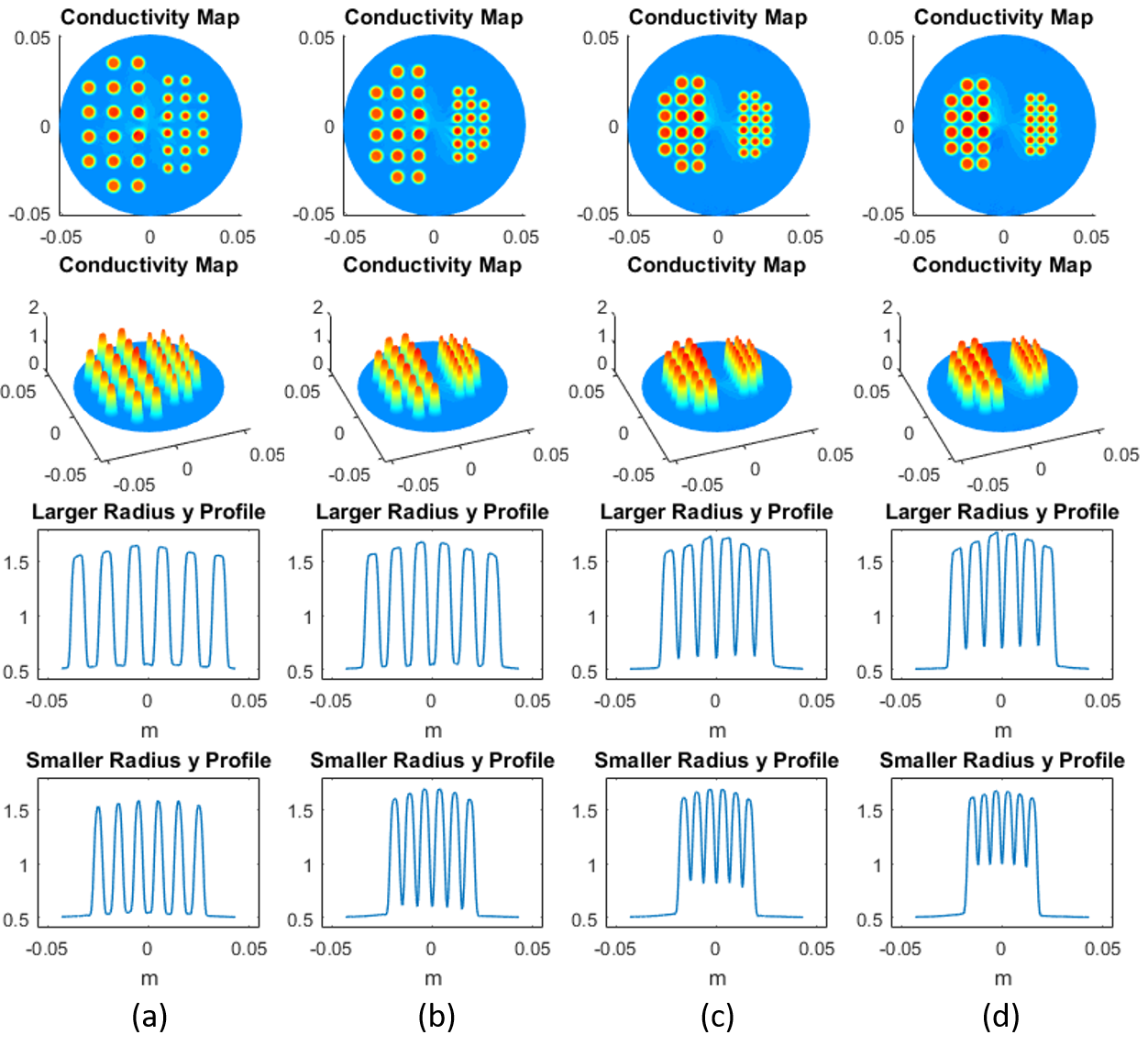
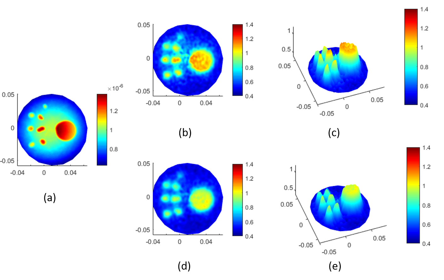
Another approach to evaluating SR is to use arrays of small objects (with 7mm and 5mm diameters) as shown in Figure-3. As the separation between them is narrowed, the reconstructed small objects interfere, but still 1 mm narrow gaps are detected. Importantly, the method does not diverge but tends to smooth the high variations.
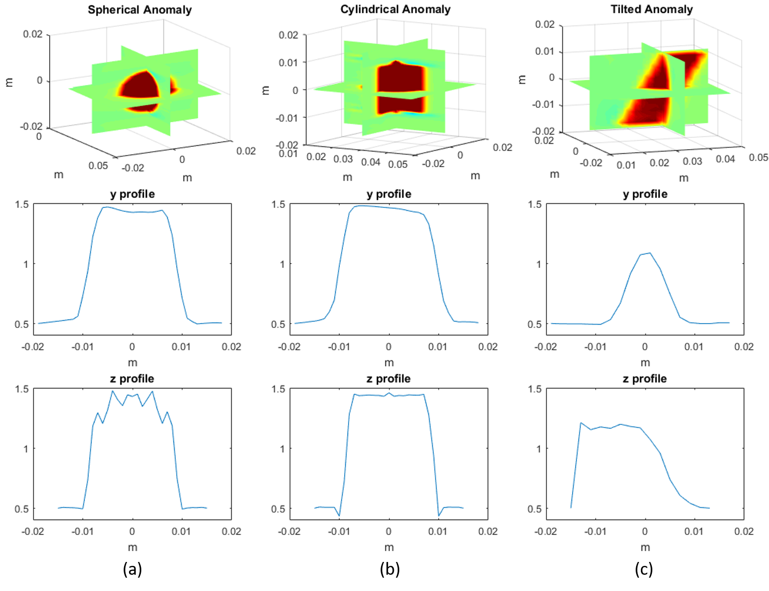
Results of simulations for 3D objects are shown in Figure-4. It is found that the performance of the method w.r.t. boundary artifact and SR is similar in the z-direction. SR is again 2-2.5 pixels in line with 2D simulations.
Results for a cylindrical experimental 2D phantom are shown in Figure-5. For $$$B_1^+$$$ phase imaging 2D SSFP is applied with QBC body coil for both transmission and reception. For $$$B_1^+$$$ magnitude mapping QBC is used for transmission and 4-channel head coil is used for reception via double angle method5. BaTiO3 pads were placed on the left or right sides to obtain two sets of data in order to apply the padding method explained previously3 to eliminate LCF artifact. Reconstructions made by combining the two data sets show good contrast and an SR similar to simulations.
Discussion and Conclusion
Full cr-MREPT has good SR which is 2-2.5 times the resolution of the MR data in case of no noise. Most of this is due to the Laplacian and derivative operators applied to $$$H^+$$$. However for noisy data 4-4.5 pixel SR values are observed mostly due to the required Low Pass Filter. Similar SR values are observed in all of x-, y-, and z-directions. It is also observed that the method yields smoothed conductivity distribution in case of variations smaller than the SR value.Acknowledgements
This study is supported by TUBITAK 114E522 grant. MR experiments are conducted in UMRAM, Bilkent, Ankara.References
1. Hafalir FS, Oran OF, Gurler N, Ider YZ. Convection-reaction equation based magnetic resonance electrical properties tomography (cr-MREPT). IEEE Trans Med Imag 2014;33:777–793.
2. Yusuf Ziya Ider, Gokhan Ariturk, and Gulsah Yildiz. Spatial and Contrast Resolution of Phase Based MREPT. Proc. Intl. Soc. Mag. Reson. Med. 24 (2016), 3642
3. Gulsah Yildiz, Gokhan Ariturk, and Yusuf Ziya Ider. Use of Padding to Eliminate Low Convective Field Artifact in Conductivity Maps Obtained by cr-MREPT. Proc. Intl. Soc. Mag. Reson. Med. 24 (2016), 1949
4. Necip Gurler and Yusuf Ziya Ider. Gradient-Based Electrical Conductivity Imaging Using MR Phase. Magn. Reson. Med. Magnetic Resonance in Medicine 77:137–150 (2016) DOI: 10.1002/mrm.26097
5. Ulrich Katscher, Dong-Hyun Kim, and Jin Keun Seo. Recent Progress and Future Challenges in MR Electric Properties Tomography. Computational and Mathematical Methods in Medicine,Volume 2013 (2013), Article ID 546562, 11 pages, http://dx.doi.org/10.1155/2013/546562
6. Gurler N, Ider YZ. Numerical methods and software tools for simulation, design, and resonant mode analysis of radio frequency birdcage coils used in MRI. Concepts Magn Reson Part B 2015;45:13–32.
7. U. Katscher, T. Voigt, C. Findeklee, P. Vernickel, K. Nehrke and O. Dossel, "Determination of Electric Conductivity and Local SAR Via B1 Mapping", IEEE Transactions on Medical Imaging, vol. 28, no. 9, pp. 1365-1374, 2009.
Figures