Synopsis

We introduce a new regularization approach, “Match Regularization”, and show that in tandem with Global Maxwell Tomography (GMT) it enables accurate, artifact-free volumetric estimation of electrical properties from noisy B1+ measurements. We demonstrated the new method for two numerical phantoms with completely different electrical properties distributions, using clinically feasible SNR levels. Estimated electrical properties were accurate throughout the volume for both phantoms. Our results suggest that GMT with match regularization is robust to noise and can be employed to map electrical properties in phantoms and in vivo experiments.

Introduction

Inverse scattering based on magnetic resonance (MR) measurements has long been considered a potential avenue for the estimation of tissue electrical properties (EP), namely relative permittivity and conductivity. Current techniques fall into two categories: local^1-3 and global^4-9 techniques. Local techniques employ the differential form of Maxwell's equations, therefore requires numerical derivatives, resulting in dramatic sensitivity to noise and inaccuracy in regions of high contrast. Global techniques employ iterative schemes based on the integral form of Maxwell's equations, which are less susceptible to noise. However, since the MR fields themselves are not sensitive to small perturbations in EP, noise can lead to several different minima. Therefore, regularization is critical for global techniques. In this work, we introduce a new regularization strategy, dubbed "Match Regularization", where the regularizer is a parameterized nonlinear function tuned to the particular problem. Our goal is to demonstrate the efficacy of this new approach in enabling EP estimation with Global Maxwell Tomography (GMT)^7-9, for clinically-achievable signal-to-noise ratio (SNR).

Theory and Methods

GMT is a fully 3D technique, which minimizes the mismatch between simulated and measured B1+ maps using the following cost function.

$$f(\epsilon)=\frac{\sqrt{\sum_k\sum_n\|w_k\odot{w}_{n}\odot\delta_{kn}\|_2^2}}{\eta}=\frac{\sqrt{\sum_k\sum_n\left\lVert{w}_{k}\odot{w}_{n}\odot\left(\hat{b}^+_k\odot\overline{\hat{b}_n^+}-b_k^+\odot\overline{b_n^+}\right)\right\rVert_2^2}}{\eta}$$

We added a second cost function to include the new regularizer, which preserves high-contrast regions and penalizes low-contrast regions:

$$f_0(\epsilon)=\frac{1}{3N_s^{\frac{2}{3}}}\sum_{\vec{n}\in S}\left(1-e^{\beta \left(\delta-\sqrt{|\Delta_x \epsilon|_{n}^2+\delta^2}\right)}\right)+\left(1-e^{\beta\left(\delta-\sqrt{|\Delta_y \epsilon|_{n}^2+\delta^2}\right)}\right)+\left(1-e^{\beta\left(\delta-\sqrt{|\Delta_z \epsilon|_{n}^2+\delta^2}\right)}\right)$$

$$$S$$$ is the set of indices comprising the scatterer and contains $$$N_s$$$ entries. $$$\Delta_\alpha$$$ denotes finite-differencing along dimension $$$\alpha$$$. $$$\beta$$$ is selected such that for a given $$$\delta$$$ and critical jump $$$|\Delta \epsilon|^\ast$$$, the gradient reaches a maximum. For $$$|\Delta\epsilon|\ll\delta$$$, the regularizer behaves like $$$\text{L}_2$$$ total variation. For $$$\delta<|\Delta\epsilon|<|\Delta\epsilon|^\ast$$$, the regularizer behaves roughly like $$$\text{L}_1$$$ total variation. Lastly, for $$$|\Delta\epsilon|>|\Delta\epsilon|^\ast$$$, the gradient of the cost function vanishes, entering a regularization regime resembling $$$\text{L}_0$$$ regularization.

The full cost function is $$$f(\epsilon) + \alpha \cdot f_0(\epsilon)$$$, where $$$\alpha$$$ is a constant weight.

We used MARIE^10,11 to iteratively simulate B1+ maps from incident fields and updated guesses material properties. The adjoint formulation of MARIE was used to calculate co-gradients analytically. The first eight components of an "ultimate basis" generated via randomized SVD¹² were employed as incident fields of a hypothetical 8-channel transmit array, in order to decouple the performance of the algorithm from the quality of the excitation. We evaluated our technique using two numerical phantoms with asymmetric EP distributions: a four-compartment tissue-mimicking phantom and a torso-mimicking phantom. The latter was chosen because accurate estimation of its EP from noisy data has failed using local techniques². We performed numerical GMT experiments using a homogeneous initial guess (i.e., worst case scenario) for different noise levels in the synthetic B1+ maps. We characterized noise in the data using peak SNR (pSNR), defined as

$$\text{SNR}_k=\frac{\|b_k^+\|_\infty}{\sigma}$$

where $$$\sigma$$$ is the standard deviation of the additive Gaussian noise. We believe that this is the most robust SNR metric, since mean SNR (mSNR) could result in regions with unrealistically large SNR for multiple channel transmission.

Results

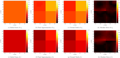
Through trial and error, we were able to "match" our regularizer to the four-compartment phantom at 6mm resolution, with $$$\delta=0.1$$$, $$$|\Delta\epsilon|^\ast=1.5$$$ and $$$\alpha=10^{-2}$$$. Figure 1 shows initial guess, estimated EP, ground truth, and absolute error, for pSNR=50, corresponding to mSNR of 15-27.

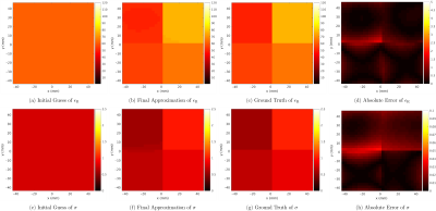
The peak/mean error over the entire volume was 2.4/0.47% for relative permittivity and 4.6/1% for conductivity. For higher SNRs, errors were slightly smaller, whereas reconstructions were perfect at every voxel in the absence of noise (not shown). Figure 2 shows the results for 3mm resolution, reusing the same regularization parameters. Peak/mean error was 3.4/0.55% and 8.3/1.4% for relative permittivity and conductivity, respectively. For the torso-mimicking phantom (10mm resolution) we used pSNR=200, corresponding to mSNR of 13-28 and kept $$$\delta$$$ and $$$|\Delta\epsilon|^\ast$$$ as for the other phantom, but we set $$$\alpha$$$ to $$$8\cdot{10}^{-4}$$$. Figure 3 shows the results, after clustering the material properties⁹, in which peak/mean error was 0.4/0.2% and 0.36/0.28% for relative permittivity and conductivity, respectively.

Discussion and Conclusion

Acknowledgements

References

1. U. Katscher, T. Voigt, C. Findeklee, P. Vernickel, K. Nehrke, and O. Dossel, “Determination of Electric Conductivity and Local SAR Via B1 Mapping,”IEEE Trans. Med. Imaging, vol. 28, no. 9, pp. 1365–1374, Aug. 2009.
2. D.K. Sodickson, L. Alon, C.M. Deniz, R. Brown, B. Zhang, G.C. Wiggins, G.Y. Cho, N.B. Eliezer, D.S. Novikov, R. Lattanzi, Q. Duan, L. Sodickson and Y. Zhu. Local Maxwell tomography using transmit-receive coil arrays for contact-free mapping of tissue electrical properties and determination of absolute RF phase; 20th Scientic Meeting of the International Society for Magnetic Resonance in Medicine (ISMRM). Melbourne (Australia), 5-11 May 2012, p. 387.
3. J.P. Marques, D.K. Sodickson, O. Ipek, C.M. Collins, and R. Gruetter, “Single acquisition electrical property mapping based on relative coil sensitivities: A proof-of-concept demonstration,” Magn. Reson. Med., vol. 74, no. 1, pp. 185–195, Aug. 2014.
4. J. Liu, X. Zhang, S. Schmitter, P.-F. Van de Moortele, and B. He, “Gradient-based electrical properties tomography (gEPT): A robust method for mapping electrical properties of biological tissues in vivo using magnetic resonance imaging,” Magn. Reson. Med., vol. 74, no. 3, pp. 634–646, Sep. 2014.
5. E. Balidemaj, C. A. T. van den Berg, J. Trinks, A. L. van Lier, A. J. Nederveen, L. J. Stalpers, H. Crezee, and R. F. Remis, “CSI-EPT: A Contrast Source Inversion Approach for Improved MRI-Based Electric Properties Tomography,” IEEE Trans. Med. Imaging, vol. 34, no. 9, pp. 1788–1796, Aug. 2015.
6. R.F. Remis, A.W.S. Mandija, R.L. Leijsen, P.S. Fuchs, P.R.S. Stijnman, & C.A.T. van den Berg. Electrical properties tomography using contrast source inversion techniques. In Electromagnetics in Advanced Applications (ICEAA), 2017 International Conference on (pp. 1025-1028). IEEE, Sep. 2017.
7. J. E. C. Serralles, A. G. Polymeridis, M. Vaidya, G. Haemer, J.K. White, D. K. Sodickson, L. Daniel and R. Lattanzi, “Global Maxwell Tomography: a novel technique for electrical properties mapping without symmetry assumptions or edge artifacts,” 24th Scientific Meeting of the International Society for Magnetic Resonance in Medicine (ISMRM). Singapore, 7-13 May 2016, p. 2993.
8. J.E.C. Serrallés, L. Daniel, J.K. White, D.K. Sodickson, R. Lattanzi, & A.G. Polimeridis. Global Maxwell Tomography: A novel technique for electrical properties mapping based on MR measurements and volume integral equation formulations. In Antennas and Propagation (APS-URSI), 2016 IEEE International Symposium on (pp. 1395-1396).
9. J.E.C. Serralles, I. Georgakis, A.G. Polimeridis, L. Daniel, J.K. White, D.K. Sodickson, and R. Lattanzi. "Volumetric Reconstruction of Tissue Electrical Properties from B1+ and MR Signals Using Global Maxwell Tomography: Theory and Simulation Results." 25th Scientific Meeting of the International Society for Magnetic Resonance in Medicine (ISMRM). Hawaii, 22-27 April 2017, p. 3647.
10. J.F. Villena, A.G. Polimeridis, Y. Eryaman, E. Adalsteinsson, L.L. Wald, J.K. White, and L. Daniel. “Fast electromagnetic analysis of MRI transmit RF coils based on accelerated integral equation methods.” IEEE Transactions on Biomedical Engineering, 63 (11): 2250-2261, 2016.
11. A.G. Polimeridis, J.F. Villena, L. Daniel, J.K. White. “Stable FFT-JVIE solvers for fast analysis of highly inhomogeneous dielectric objects,” Journal of Computational Physics, Volume 269, 15 July 2014, Pages 280-296, ISSN 0021-9991, http://dx.doi.org/10.1016/j.jcp.2014.03.026.
12. N. Halko, P.G. Martinsson, & J.A. Tropp. (2011). Finding structure with randomness: Probabilistic algorithms for constructing approximate matrix decompositions. SIAM review, 53(2), 217-288.