Synopsis

Contrast Source Inversion Electrical Properties Tomography (CSI-EPT) is an integral-based method that aims to reconstruct tissue electrical properties through an iterative minimization procedure. This method requires complex $$$B_1^+$$$ data as input. In practice, however, the transmit phase cannot be measured in MRI-experiments. Only the transceive phase can be calculated from MR-measurements. In this work, the CSI-EPT reconstruction algorithm is reformulated to take the transceive phase into account. This transceive phase correction opens the possibility to exploit higher sensitivity of EPT at higher field strengths with regular quadrature setups. Additionally, for the first time CSI-EPT reconstructions from MR-measurements are shown.

Introduction

Helmholtz-based MR-Electrical-Properties-Tomography (MR-EPT) is a derivative-based approach that reconstructs tissue electrical properties (EPs: conductivity σ, permittivity ε) directly from MR-measurements. MR-EPT reconstructions are highly sensitive to noise and present severe boundary artifacts¹.

Alternatively, Contrast-Source-Inversion-EPT (CSI-EPT), an integral-based approach, is less sensitive to noise and boundary artifacts². CSI-EPT requires complex $$$B_1^+$$$ data. However, $$$B_1^+$$$ phase measurements are not possible in practice. Here, the standard CSI-EPT algorithm² has been reformulated in terms of the accessible transceive phase, and first reconstructions from MR-measurements are presented.

Methods

The original CSI-EPT method attempts to find tissue EPs by minimizing the cost functional²

$$F(w_j,\chi)=\eta_S\sum\limits_j||B_{1,j}^{+;sc}-G_S\{w_j\}||_S^2+\eta_D\sum\limits_j||{\chi}E_{j}^{inc}-w_j+{\chi}G_D\{w_j\}||_D^2,\quad\quad\quad(1)$$

where the contrast source $$$w_j={\chi}E_j$$$ (with the contrast function $$$\chi(\mathbf{x})=\epsilon_r(\mathbf{x})-1+\frac{\sigma(\mathbf{x})}{i\omega\epsilon}$$$) and $$$E_j$$$ the electric field corresponding to the jth antenna setting operating at the Larmor frequency $$$\omega$$$), $$$\eta_{S,D}$$$ normalization factors, $$$G_S$$$ the data operator mapping contrast sources to scattered $$$B_1^+$$$ data, $$$G_D$$$ the object operator mapping contrast sources to electric fields, $$$B_{1,j}^{+;sc}=B_{1,j}^{+}-B_{1,j}^{+;inc}$$$ the scattered $$$B_1^+$$$ field, while $$$E_j^{inc}$$$ and $$$B_{1,j}^{+;inc}$$$ are the fields in an empty coil, obtainable through simulations or measurements.

The MR-accessible transceive phase is the sum of the transmit/receive phases, $$$\phi_+$$$/$$$\phi_-$$$, respectively. To obtain $$$\phi_+$$$, the transceive-phase-assumption³ (TPA) is often used:

$$\phi_+=\phi_-=\frac{\phi_{\pm}}{2}\quad\quad\quad(2) $$

This assumption breaks down for increasing field strengths and non-symmetrical objects. Here, the CSI-EPT formalism is rewritten to include the measured transceive phase:

$$F(w_j,\chi,\phi_-)=\eta_S\sum\limits_j||{\color{blue}{|B_{1,j}^{+}|e^{i\phi_{\pm}}}}e^{-i\phi_-}-G_S^+\{w_j\}-{\color{blue}{B_1^{+;inc}}}||_S^2+\eta_D\sum\limits_j||\chi{\color{blue}{E_{j}^{inc}}}-w_j+{\chi}G_D\{w_j\}||_D^2, \quad\quad\quad(3) $$

where the $$$B_1^+$$$ field is given in polar form, the transmit phase is written in terms of the transceive (known) and receive (unknown) phases (input data are indicated in blue).

Here, the receive phase is iteratively updated using the current estimates of the contrast function and electric field. Specifically, the scattered receive field is computed at each iteration, n, using

$$B_{1,n}^{-,sc}=G_S\{\chi_{n-1}E_n^{RE}\}, \quad\quad\quad(4) $$

where $$$E_n^{RE}$$$, the electric field during reception, is:

$$E_n^{RE}=G_D\{\chi_{n-1}E_n^{RE}\}+E^{inc;RE}. \quad\quad\quad(5) $$

$$$E^{inc;RE}$$$, the incident electric field, is modelled together with $$$B_1^{-inc,RE}$$$ for an empty birdcage coil.

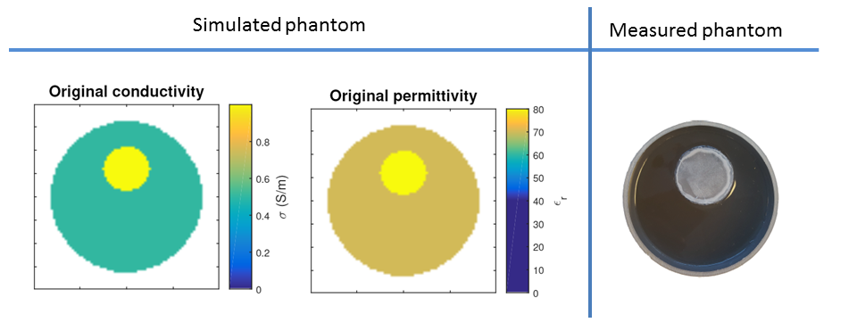
First, the impact of TPA on CSI-EPT was investigated using 2D-line source simulations (Matlab), mimicking the center plane of a birdcage coil. The field distributions were computed using the phantom contrast (Fig.1) and used as input for CSI-EPT reconstructions. Comparison between the EPs reconstructions from TPA (eq.1) and Transceive-Phase-Corrected (TPC, eq.3) was therefore performed.

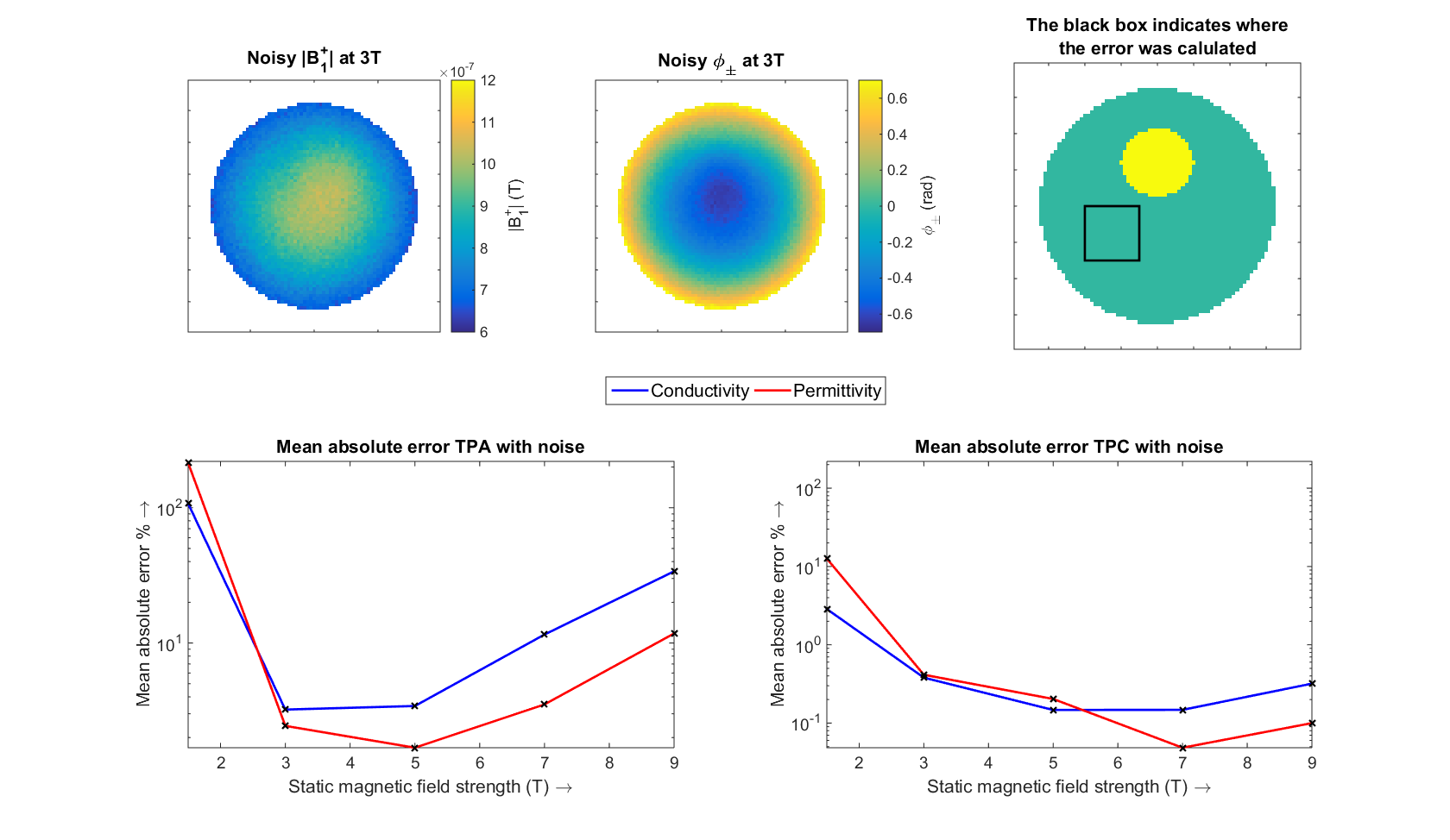
Furthermore, the impact of noise and field strength was also investigated with realistic Signal-to-Noise-Ratio (SNR) values⁴.

Additionally, 3D-FDTD simulations (Sim4Life, ZMT, CH) were performed modeling a 68 cm 3T birdcage coil. Finally, comparison between CSI-EPT and MR-EPT conductivity reconstructions was performed.

MR-measurements (3T, Ingenia, Philips, Netherlands) were conducted using the body/head-coils for transmission/reception, respectively. The $$$B_1^+$$$ magnitude was measured with an AFI sequence⁵. The transceive phase was computed by combining two Spin-Echo sequences with opposite readout polarities³, and by compensating for the head coil receive sensitivity using an available vendor specific algorithm (CLEAR).

Results & Discussion

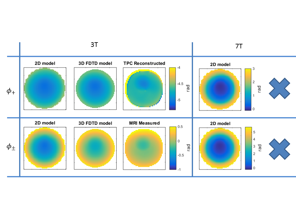
Figure 2 shows $$$\phi_+$$$ and $$$\frac{\phi_{\pm}}{2}$$$ from simulations, measurements and reconstructions. The reconstructed $$$\phi_+$$$ from MR-measurements resembles well the simulated $$$\phi_+$$$ even though the transceive phase in the 2D-model has a bigger curvature.

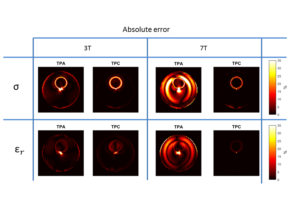
Figure 3 shows the absolute error in conductivity and permittivity reconstructions at 3T and 7T assuming noiseless input data for TPA and TPC. For TPA, the EPs reconstruction error increases with the field strength. If TPC is used, this error is strongly reduced.

Figure 4 shows that the error in CSI-EPT reconstructions is due to noise at low field strengths, whereas it is mainly due to the TPA at higher field strengths. If TPC is used, the reconstruction error decreases with increasing field strength, which is due to the intrinsic increase in SNR and RF field curvature.

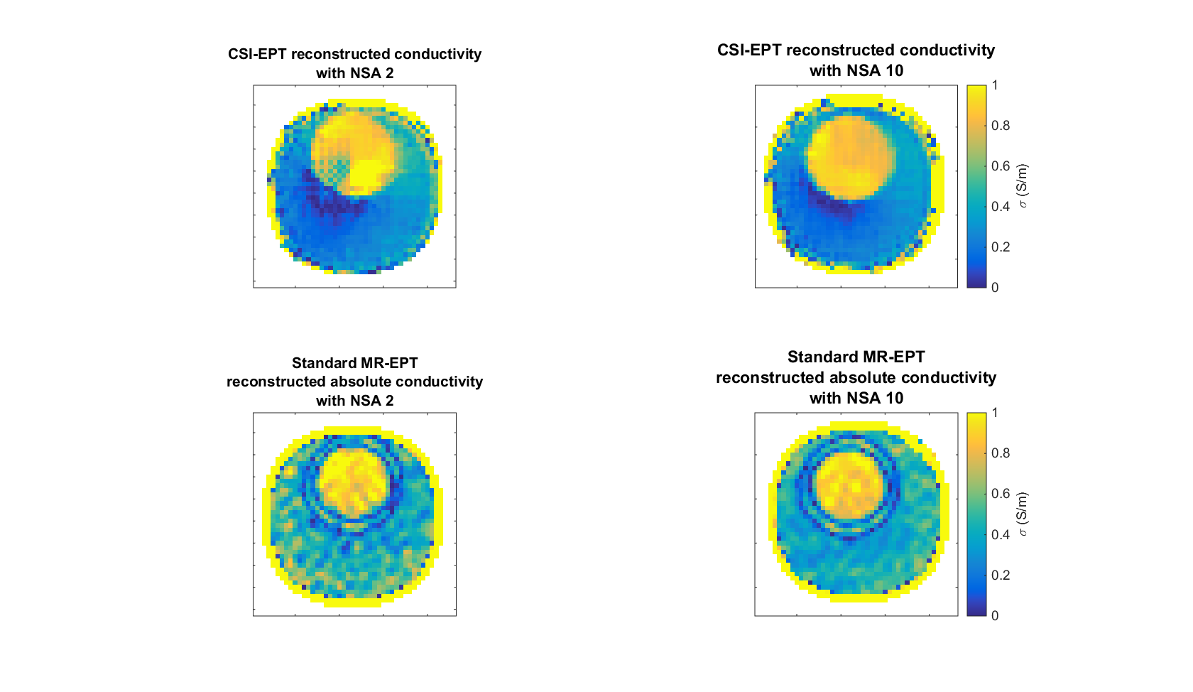
Figure 5 shows that MR-EPT reconstructions are highly sensitive to noise (even if high NSA is used), while CSI-EPT reconstructions are more noise-robust. CSI-EPT suffers less from boundary issues compared to MR-EPT. However, CSI-EPT suffers from inaccuracies where the electric field is small (center of the phantom). CSI-EPT permittivity reconstructions (not shown) were not representative, most likely due to a mismatch between the modeled incident fields and the incident fields in the MR-experiment. This mismatch can be considered a systematic error to be further investigated.

Conclusion

Acknowledgements

References

[1] S. Mandija, A.Sbrizzi, P.R. Luijten, and C.A.T. van den Berg, “Error analysis of Helmholtz-based MR-Electrical Pproperty Tomography”, Magnetic Resonance in Medicine,2017;early view. doi:10.10002/mrm.27004.

[2] E. Balidemaj, C.A.T. van den Berg, J. Trinks, A.L.H.M.W. van Lier, A.J. Nederveen, L.J.A. Stalpers, H.Crezee, and R.F. Remis, “CSI-EPT: A Contrast Source Inversion Approach for Improved MRI-Based Electric Properties Tomography,” IEEE Transactions on Medical Imaging,2015;1788–1796.

[3] A.L.H.M.W. van Lier, D.O. Brunner, K.P. Pruessmann, D.W.J. Klomp, P.R. Luijten, J.J.W. Lagendijk, and C.A.T. van den Berg, “B1+ phase mapping at 7 T and its application for in vivo electrical conductivity mapping,” Magnetic Resonance in Medicine,2012; 552–561.

[4] C.M. Collins and M.B. Smith, “Signal-to-noise ratio and absorbed power as functions of main magnetic field strength, and definition of rf pulse for the head in the birdcage coil”, Magnetic Resonance in Medicine,2001;684–691. doi:10.1002/mrm.1091.

[5] V.L. Yarnykh, “Actual flip-angle imaging in the pulsed steady state: A method for rapid three-dimensional mapping of the transmitted radiofrequency field”, Magnetic Resonance in Medicine,2007;192–200.