5086
Diffusion Tensor Magnetic Resonance Electrical Impedance Tomography versus Magnetic Resonance Conductivity Tensor Imaging1Electrical and Electronics Engineering, METU, Ankara, Turkey
Synopsis
In this study, recently proposed diffusion tensor magnetic resonance electrical impedance tomography (DT-MREIT) is compared with magnetic resonance conductivity tensor imaging (MRCTI) using simulated measurements generated by means of a finite element model. Both methods are used to reconstruct conductivity tensor images of an anisotropic conductivity distribution. In DT-MREIT, extra cellular conductivity and diffusivity ratio (ECDR) is recovered from its transverse gradient. In MRCTI, the conductivity tensor is reconstructed from two current profiles by using anisotropic Bz sensitivity (ABzS) method with a stronger regularization. Reconstructed conductivity images suggest that MRCTI provides better accuracy than DT-MREIT, at lower SNR levels.
Introduction
DT-MREIT method uses diffusion tensor images along with current density images of the same object to obtain conductivity tensor images 1. In this method, the linear relation between the conductivity $$$\overline{\overline{\sigma}}$$$ and diffusion $$$\overline{\overline{D}}$$$ tensors in a porous medium is exploited 2.
$$\overline{\overline\sigma}={\bf{H}_{\it{ext}}}\overline{\overline{D}}\space\space\space[1]$$
where $$${\bf{H_{\it{ext}}}}$$$ is called the extra cellular conductivity and diffusivity ratio (ECDR).
To obtain the distribution of $$${\bf{H_{\it{ext}}}}$$$, at least two linearly independent current patterns are injected to the imaging region. The resulting current density distribution is given by:
$${\bf{J_{\it{i}}}}={-\overline{\overline{\sigma}}\triangledown{\bf{\Phi_{\it{i}}}}}=-{\bf{H_{\it{ext}}}}\overline{\overline{\it{D}}}\triangledown{\bf\Phi_{\it{i}}}\space\space\space\space{\it{i=1,\space2}}\space\space\space[2]$$
where $$$\bf{\Phi}$$$ is the electrical potential. The curl-free condition of electric field at low frequencies 3 results in:
$$\triangledown\times({\overline{\overline{D}}^{\space{-1}}}{\bf{J_{\it{i}})}}=\triangledown{ln\bf{{H_{\it{ext}}}}}\times({\overline{\overline{D}}^{\space{-1}}}{\bf{J_{\it{i}})}}\space\space{\it{i=1,\space2}}\space\\\triangledown{ ln\bf{{H_{\it{ext}}}}}=\begin{bmatrix}\frac{\partial{\it{ln\bf{H_{\it ext}}}}}{\partial{\it{x}}}\\\frac{\partial{\it{ln\bf{{H_{\it{ext}}}}}}}{\partial\bf{\it{y}}}\end{bmatrix}\space\space\space[3]$$
For the two linearly independent current injection profiles, Eq. [3] can be expressed in matrix form 3:
$$\begin{bmatrix}{\overline{\overline{D}}^{\space{-1}}\bf{J_{\it{y,1}}}}&{-\overline{\overline{D}}^{\space{-1}}\bf{J_{\it{x,1}}}}\\{\overline{\overline{D}}^{\space{-1}}\bf{J_{\it{y,2}}}}&-{\overline{\overline{D}}^{\space{-1}}\bf{J_{\it{x,2}}}} \end{bmatrix}\begin{bmatrix}\frac{\partial{ln\bf{H}_{\it{ext}}}}{\partial{\it{x}}}\\\frac{\partial{ln\bf{H}_{\it{ext}}}}{\partial{\it{y}}}\end{bmatrix}=\begin{bmatrix}\frac{\partial{({\overline{\overline{D}}^{\space{-1}}\bf{J_{\it{x,1}}}})}}{\partial{\it{y}}}-\frac{\partial{({\overline{\overline{D}}^{\space{-1}}\bf{J_{\it{y,1}}}})}}{\partial{\it{x}}}\\\frac{\partial({\overline{\overline{D}}^{\space{-1}}\bf{J_{\it{x,2}}}})}{\partial{\it{y}}}-\frac{\partial({\overline{\overline{D}}^{\space{-1}}\bf{J_{\it{y,2}}}})}{\partial{\it{x}}}\end{bmatrix}\space\space\space[4]$$
By solving this equation, $$$\triangledown{ln\bf{H}_{\it{ext}}}$$$ is obtained. To recover $$${ln\bf{H}_{\it{ext}}}$$$ from $$$\triangledown{ln\bf{H}_{\it{ext}}}$$$ two iterative methods, 1,3 have been proposed. Here, a new approach to estimate $$$\triangledown{ln\bf{H}_{\it{ext}}}$$$ by using first order discrete approximations of gradient operators is proposed. This method enables a simpler and faster reconstruction process.
In MRCTI, current induced magnetic flux density’s orthogonal component for two independent current injection profiles is obtained. Anisotropic $$$B_{z}$$$ sensitivity $$$(AB_{z}S)$$$ method, 4 is used to reconstruct anisotropic conductivity image. This method is based on finding perturbation of conductivity tensor $$$\triangle{\overline{\overline{\sigma}}}$$$ for a given perturbation $$$\triangle\bf{b}$$$ in the orthogonal component of magnetic flux density using:
$${\bf{S}}{\triangle{\bf{\overline{\overline\sigma}}}}=\triangle{\bf{b}}\space\space\space[5]$$
where $$$\bf{S}$$$ is the sensitivity matrix and obtained similarly to 4. To solve Eq. [5], Tikhonov regularization with smoothness prior is used as explained in the next section.
Methods
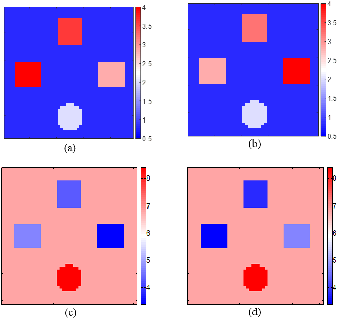
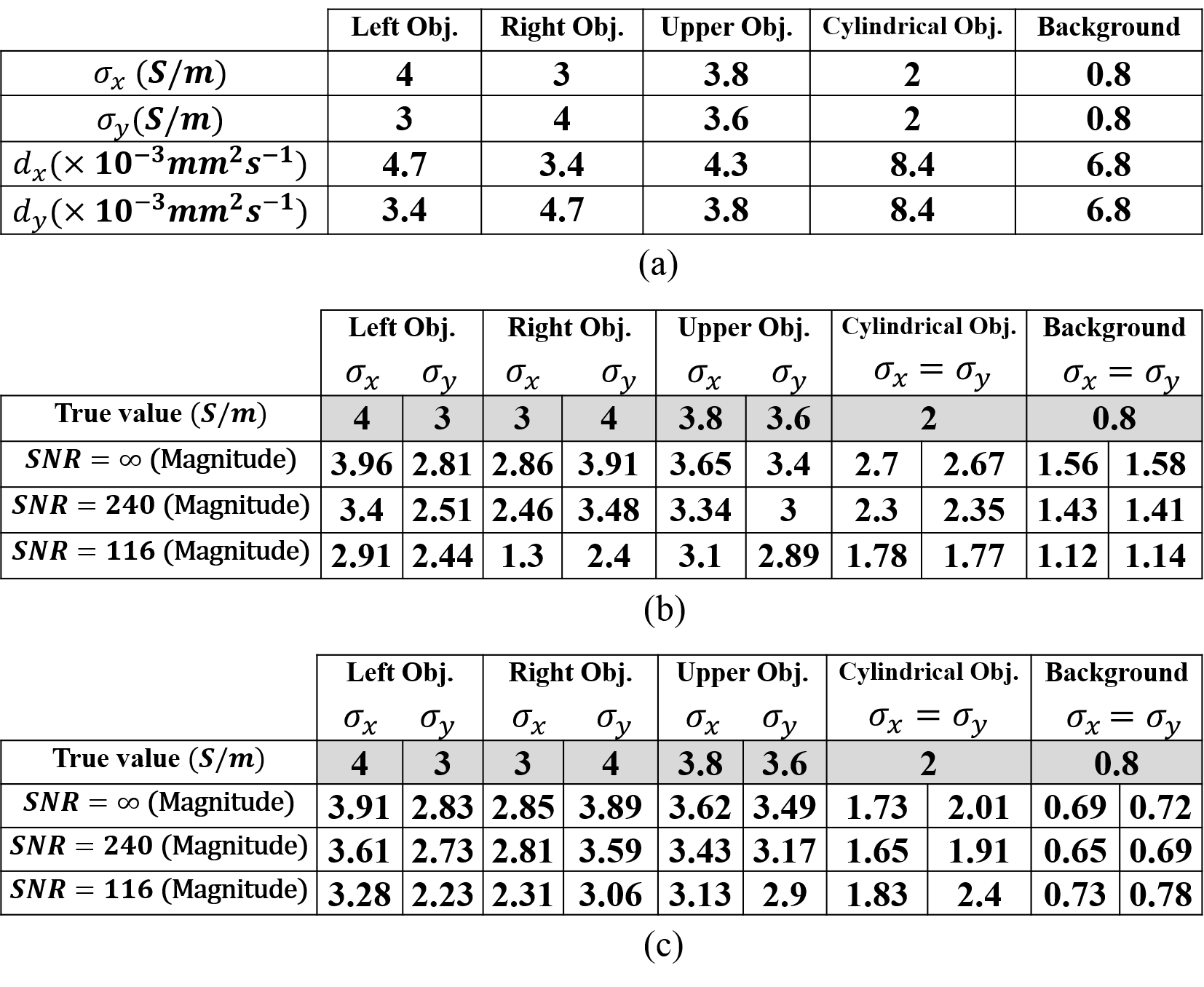
To simulate anisotropic diffusion distribution in DT-MREIT, the method proposed by Kwon et al. 1 is implemented for different values of diffusion and conductivity (Table 1(a)).
In order to recover ECDR $$$(\bf{H}_{\it{ext}})$$$ after solving the matrix equation in Eq. [4], first order discrete approximations of x and y gradient operators, i.e. $$$\bf{D}_{\it{x}}$$$ and $$$\bf{D}_{\it{y}}$$$, matrices are used 5. Hence, $$$\bf{D}_{\it{x}}{\it{ln}\bf{H}_{\it{ext}}}$$$ and $$$\bf{D}_{\it{y}}{\it{ln}\bf{H}_{\it{ext}}}$$$ are respectively discrete approximations to $$$\triangledown_{x}ln\bf{H}_{\it{ext}}$$$ and $$$\triangledown_{y}ln\bf{H}_{\it{ext}}$$$, as follows:
$$\triangledown{ln{\bf{H}_{\it{ext}}}}=\begin{bmatrix}\frac{\partial{ln{\bf{H}}_{\it{ext}}}}{\partial{\it{x}}}\\\frac{\partial{ln{\bf{H}_{\it{ext}}}}}{\partial{\it{y}}}\end{bmatrix}\approx\begin{bmatrix}{\bf{D}}_{\it{x}}\\{\bf{D}_{\it{y}}}\end{bmatrix}ln{\bf{H}}_{\it{ext}}={\bf{D}_{\it{xy}}}{\it{ln}{\bf{H}_{\it{ext}}}}\space\space\space[6]$$
Eq. [6] can be solved using least squares solution as follows:
$$ln{{\bf{H}}_{\it{ext}}}=({\bf{D}_{\it{xy}}^{\it{T}}}{\bf{D}}_{\it{xy}})^{-1}{\bf{D}}_{\it{xy}}^{\it{T}}\triangledown{\it{ln}{\bf{H}}_{\it{ext}}}\space\space\space[7]$$
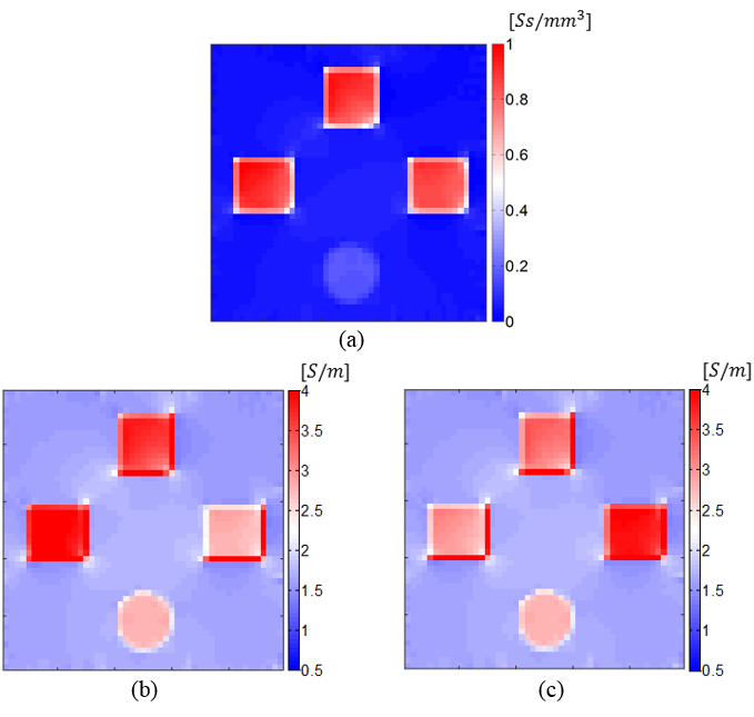
After recovering $$$ln{\bf{H}_{\it{ext}}}$$$, $$$\bf{H}_{\it{ext}}$$$ distribution can be obtained. Then, the conductivity tensor image can be reconstructed using Eq. [1] as illustrated in Fig. 2(b, c) for SNR=$$$\infty$$$.
To solve the inverse problem of MRCTI, Tikhonov regularized least squares solution with smoothness prior is used 6:
$$\begin{bmatrix}\triangle{\bf{\sigma}_{x}}\\\triangle{\bf{\sigma}_{y}}\end{bmatrix}=argmin_{\triangle{\bf{\sigma}_{x}},\triangle{\bf{\sigma}_{y}}}\mid\mid{\bf{S{\triangle{\sigma}}}_{\bf{x,y}}}-\triangle{\bf{b}}\mid\mid_{2}^{2}+\lambda(\mid\mid{\bf{D}}_{\it{xy}}\triangle{\bf{\sigma}}_{{x}}\mid\mid_{2}^{2}+\mid\mid{\bf{D}}_{\it{xy}}\triangle{\bf{\sigma}}_{y}\mid\mid_{2}^{2})=({\bf{S}^{\it{T}}S}+\lambda{\bf{D}^{\it{T}}D})^{-1}{\bf{S}}^{\it{T}}\triangle{\bf{b}}\\{\bf\triangle{\sigma}_{\bf{x,y}}}=\begin{bmatrix}\triangle{\sigma}_{\bf{x}}\\\triangle{\sigma}_{\bf{y}}\end{bmatrix}\space\space\space,\space\space\space{\bf{D}}=\begin{bmatrix}{\bf{D}}_{\it{xy}}&{0}\\{0}&{\bf{D}}_{\it{xy}}\end{bmatrix}\space\space\space[8]$$
Here, this prior information is preferred due to physical structure of the simulation model, and results in better regularization compared to using identity matrix instead of $$$\bf{D}$$$. Because the number of independent current injection profiles are reduced than before, 7 a better regularization is needed to compensate the effect of this reduction.
Results
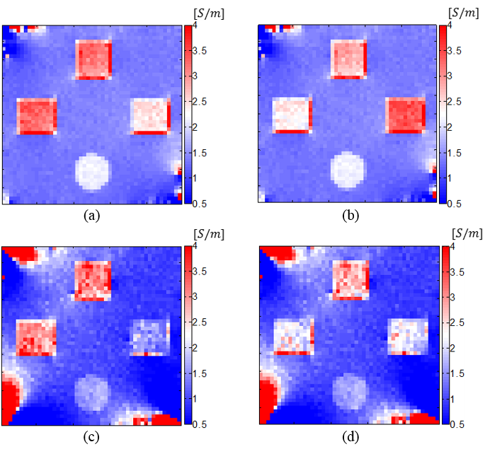
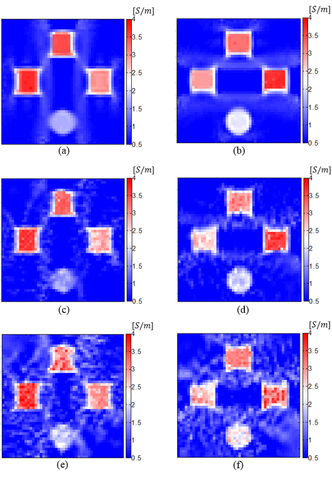
To generate simulated measurements, a finite element model of size 8cm×8cm×2cm is constructed using COMSOL (COMSOL AB, Sweden). Three similar cubic inhomogeneities of size 1.6cm×1.6cm×2cm and one cylindrical inhomogeneity with a radius of 0.8cm and a height of 2cm are placed in a background material as shown in Fig. 1. Other physical properties of the model elements are given in Table 1(a). The reconstructed conductivity distributions $$$({\bf{\sigma}}_{\it{x}}\space,\space{\bf{\sigma}}_{\it{y}})$$$ using the two imaging methods are given in Fig. 2-4 for different SNR levels. In order to evaluate the performance of the two methods the mean values of the reconstructed conductivities for each object and background are given in Table 1(b, c).Discussion and Conclusion
As shown in Fig. 3-4, the reconstructed conductivity images in DT-MREIT are nosier than those in MRCTI, at lower SNR levels. This is because in DT-MREIT noise affects both the current density and the diffusion tensor, which are then used to calculate the ECDR $$$(\bf{H}_{\it{ext}})$$$ whereas in MRCTI noise only affects $$$\triangle\bf{b}$$$ distribution. The proposed DT-MREIT reconstruction method to recover position dependent ECDR results in acceptable conductivity images in SNR=240 with less than 18% reconstruction error. However, for reduced SNR level the reconstructed conductivity images have artifacts, especially at the corners of the field of view due to the lower current densities in those regions. Nevertheless, the inhomogeneities are still distinguishable with sharp edges. Performance of MRCTI is better than DT-MREIT at lower SNRs. Using a stronger prior information in inverse problem of MRCTI helps to improve the reconstruction despite using a fewer number of current injection profiles. Moreover, the artifacts in the reconstructed images may be due to model mismatches in the forward problem. These artifacts can be reduced by increasing the discretization level i.e. by using a larger $$$\bf{S}$$$ matrix. However, by increasing discretization in the field of view pixel dimension reduces which results in a lower SNR.Acknowledgements
Mehdi Sadighi is a Ph.D. student at Middle East Technical University under the supervision of B. Murat Eyuboglu. This study is funded by The Scientific and Technological Research Council of Turkey (TÜBİTAK) under Research Grant 116E157.References
1. Kwon OI, Jeong WC, et al. Anisotropic conductivity tensor imaging in MREIT using directional diffusion rate of water molecules, Phys. Med. Biol., 2014;59(12):2955-2974.
2. Tuch DS, Wedeen V J, Dale AM, George J S and Belliveau J W. Conductivity tensor mapping of the human brain using diffusion tensor MRI Proc. Natl Acad. Sci. USA 2001, 11697–11701
3. Jeong WC, Sajib SZ, Katoch N, Kim HJ, Kwon OI, Woo EJ. Anisotropic conductivity tensor imaging of in vivo canine brain using DT-MREIT. IEEE Trans Med Imaging. 2017;36:124–131.
4. Değirmenci E, Eyüboğlu BM. Image reconstruction in magnetic resonance conductivity tensor imaging (MRCTI), IEEE Trans. Med. Imaging, 2012 ;31(3):525-532.
5. Sharif B, Kamalabadi F. Optimal Sensor Array Configuration in Remote Image Formation, IEEE Transactions on Image Processing, 2008;17(2):155-166.
6. Hansen PC. Discrete inverse problems: insight and algorithms, 2010. SIAM.
7. Değirmenci E, Eyüboğlu BM. Practical realization of magnetic resonance conductivity tensor imaging (MRCTI) IEEE Trans. Med. Imaging, 2013 ; 32:601–608.
8. Oran ÖF, İder YZ. Feasibility of conductivity imaging using subject eddy currents induced by switching of MRI gradients, Magn. Reson. Med., 2017;77(5):1926-1937.
Figures